Inventory is the goods and materials a business holds for sale, for use in producing goods for sale, or for consumption in the production process. Depending on the business, inventory can include merchandise, raw materials, work in process, and finished goods.
Inventory is an asset while the related goods remain unsold. When inventory is sold, its applicable recorded cost generally moves into cost of goods sold, which affects the income statement.
This makes inventory both an accounting asset and an operational resource. Too little inventory can create stockouts and lost sales, while too much can tie up cash and increase storage, financing, shrinkage, and obsolescence costs.
What Is Inventory?
Inventory represents goods or materials held as part of a company’s ordinary operating cycle.
For a retailer, inventory may consist primarily of merchandise purchased for resale.
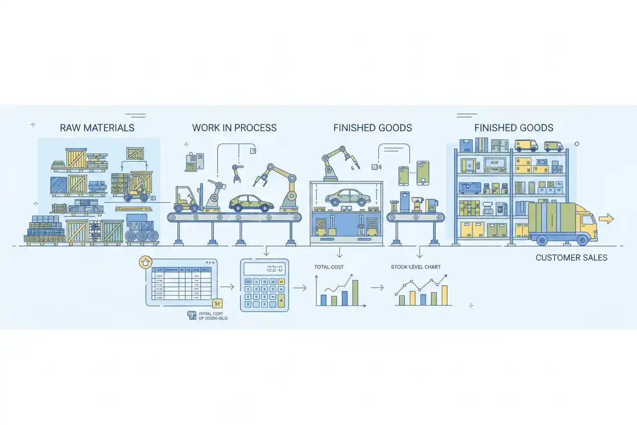
For a manufacturer, inventory can exist at several stages:
Raw materials are inputs not yet placed into production.
Work in process consists of partially completed products.
Finished goods are completed products waiting to be sold.
The amount and composition of inventory can therefore differ significantly across industries.
A consulting firm may carry very little physical inventory, while a retailer, manufacturer, distributor, or wholesaler can have a large portion of its working capital tied up in stock.
Inventory Formula
A basic inventory flow formula is:
Ending Inventory = Beginning Inventory + Inventory Purchases or Production Additions − Cost of Inventory Sold or Used
For a merchandising business under a simplified periodic framework:
Ending Inventory = Beginning Inventory + Purchases − Cost of Goods Sold
The same relationship can be rearranged to calculate COGS:
Cost of Goods Sold = Beginning Inventory + Purchases − Ending Inventory
Suppose a retailer begins with $80,000 of inventory, purchases another $420,000, and records $390,000 of COGS.
Ending inventory is:
Ending Inventory = $80,000 + $420,000 − $390,000
Ending Inventory = $110,000
The company ends the period with $110,000 of inventory under these simplified assumptions.
Inventory Example
Assume a retailer has:
| Inventory Item | Amount |
|---|---|
| Beginning inventory | $50,000 |
| Purchases | $250,000 |
| Goods available for sale | $300,000 |
| Ending inventory | $70,000 |
First calculate goods available for sale:
Goods Available for Sale = $50,000 + $250,000 = $300,000
Then determine the portion assigned to goods sold:
COGS = $300,000 − $70,000 = $230,000
The accounting relationship is therefore:
$50,000 + $250,000 = $230,000 + $70,000
The $230,000 assigned to sold merchandise becomes COGS.
The remaining $70,000 stays in inventory.
Why Inventory Is an Asset
Inventory is generally recorded as an asset because it represents economic resources expected to generate future benefit through sale or production.
Suppose a retailer purchases merchandise costing $20,000 and has not sold any of it by the reporting date.
The company has exchanged one asset—cash or a receivable-like funding source—for another asset—inventory.
The unsold merchandise does not automatically become an immediate $20,000 cost of goods sold.
When the merchandise is eventually sold, the cost assigned to those goods can move from inventory to COGS under the applicable accounting method.
Inventory on the Balance Sheet
Inventory generally appears among current assets on the balance sheet when it is expected to be sold or consumed within the normal operating cycle.
Suppose a business reports:
- Cash: $100,000
- Accounts receivable: $150,000
- Inventory: $250,000
- Other current assets: $50,000
Total current assets are:
$100,000 + $150,000 + $250,000 + $50,000 = $550,000
Inventory therefore represents approximately:
$250,000 ÷ $550,000 × 100 ≈ 45.45%
of current assets in this example.
For inventory-heavy businesses, changes in stock can therefore materially affect the balance sheet.
Inventory and the Income Statement
Inventory itself is not ordinarily shown as a sales expense merely because it exists.
Its cost generally reaches the income statement when the related goods are sold.
Suppose inventory costing $30,000 is sold for $50,000.
The simplified economics are:
Revenue = $50,000
COGS = $30,000
Gross Profit = $50,000 − $30,000 = $20,000
The sale reduces inventory by the cost assigned to the goods and recognizes that amount as COGS.
This creates a direct connection between inventory accounting and profitability.
Raw Materials Inventory
Raw materials are inputs purchased or held for production but not yet placed into the manufacturing process.
Examples could include metal used in machinery, fabric used in clothing, ingredients used in food production, or components used in electronics.
Suppose a manufacturer begins the month with $40,000 of raw materials, purchases $100,000, and transfers $90,000 into production.
Ending raw-material inventory is:
$40,000 + $100,000 − $90,000 = $50,000
The $50,000 remains in raw-material inventory at period end under the simplified example.
Work-in-Process Inventory
Work in process, or WIP, represents partially completed goods.
A product may have consumed materials, labor, and manufacturing overhead while still being unfinished at the reporting date.
Suppose:
Beginning WIP = $30,000
Production Costs Added = $200,000
Cost Transferred to Finished Goods = $190,000
Then:
Ending WIP = $30,000 + $200,000 − $190,000 = $40,000
The $40,000 represents cost associated with production that has started but has not yet become finished goods.
Finished-Goods Inventory
Finished goods are completed products that have not yet been sold.
Suppose:
Beginning Finished Goods = $60,000
Cost of Goods Manufactured = $400,000
COGS = $380,000
Then:
Ending Finished Goods = $60,000 + $400,000 − $380,000 = $80,000
The $80,000 remains as finished-goods inventory awaiting future sale.
Merchandise Inventory
Retailers and wholesalers often use merchandise inventory rather than the raw-material/WIP/finished-goods structure of manufacturers.
Suppose a retailer buys finished products from suppliers for resale.
If:
Beginning Merchandise Inventory = $100,000
Purchases = $600,000
Ending Merchandise Inventory = $150,000
then:
COGS = $100,000 + $600,000 − $150,000 = $550,000
The retailer sold inventory carrying a cost of $550,000 during the period.
Average Inventory Formula
When inventory levels fluctuate, analysts often use average inventory for certain performance calculations.
A simple two-point average is:
Average Inventory = (Beginning Inventory + Ending Inventory) ÷ 2
Suppose beginning inventory is $120,000 and ending inventory is $180,000:
Average Inventory = ($120,000 + $180,000) ÷ 2 = $150,000
This simple average is useful when beginning and ending balances reasonably represent the period.
Highly seasonal businesses may need more frequent observations because two endpoints can hide major fluctuations during the year.
Inventory Turnover
Inventory turnover uses inventory and COGS to evaluate how frequently inventory is sold or used relative to the average stock held.
A commonly used relationship is:
Inventory Turnover = Cost of Goods Sold ÷ Average Inventory
Suppose:
COGS = $900,000
Average Inventory = $150,000
Then:
Inventory Turnover = $900,000 ÷ $150,000 = 6 times
The turnover calculation has its own analytical intent. Inventory itself remains the underlying asset balance being managed.
Inventory Carrying Cost
Holding inventory is not free.
Inventory carrying cost can include relevant storage, insurance, handling, financing, shrinkage, obsolescence, deterioration, and opportunity costs associated with stock.
Suppose average inventory is $500,000 and the business estimates an annual carrying-cost rate of 20%.
A simplified carrying-cost estimate is:
Annual Inventory Carrying Cost = $500,000 × 20% = $100,000
This does not mean inventory itself is a $100,000 expense.
The carrying-cost calculation estimates the economic cost of maintaining that level of inventory.
Too Much Inventory
Excess inventory can create several problems.
Cash is tied up in products that have not yet been converted into sales.
Storage requirements increase.
Insurance, handling, shrinkage, and obsolescence exposure can rise.
Products can become outdated, damaged, unfashionable, or unsellable.
Inventory-heavy businesses should therefore evaluate both product availability and the cost of carrying stock.
A warehouse full of products is not automatically a sign of financial strength.
Too Little Inventory
Reducing inventory too aggressively creates a different set of risks.
The business may run out of stock when customers want to buy.
Production can stop if required materials are unavailable.
Emergency purchasing and expedited freight can increase costs.
Customers may switch to competitors if items are repeatedly unavailable.
Inventory management therefore involves balancing availability with the financial and operational costs of holding stock.
Economic Order Quantity and Inventory
Economic order quantity addresses how many units a business should order under a specific ordering-cost and holding-cost model.
Suppose a company uses 10,000 units annually.
Ordering extremely large quantities reduces the number of orders but increases average cycle inventory.
Ordering extremely small quantities lowers average inventory but increases ordering frequency.
EOQ seeks the cost-minimizing order size under its assumptions.
Inventory is the asset being managed; EOQ is one specialist model used to manage replenishment quantity.
Reorder Point and Inventory
A reorder point answers a different question:
At what inventory level should another order be placed?
A company might order 1,000 units at a time but trigger the order when available inventory falls to 300 units.
The 1,000-unit amount is the replenishment quantity.
The 300-unit threshold is the reorder point.
Keeping those concepts separate prevents order size and order timing from being confused.
Safety Stock and Inventory
Safety stock is additional inventory carried to protect against uncertainty.
Suppose normal expected demand during supplier lead time is 400 units, but management chooses to maintain another 100 units as a buffer.
That additional 100 units is safety stock.
It can reduce the risk of a stockout, but it also increases average inventory and therefore can raise carrying costs.
The appropriate buffer depends on demand variability, lead-time uncertainty, service requirements, and the cost of running out.
Inventory and Gross Burn
Inventory purchases can consume substantial cash and therefore affect gross burn for cash-planning purposes.
Suppose a retailer pays cash for $200,000 of inventory in March but sells only $80,000 of the related product cost during that month.
The $200,000 purchase affects cash immediately.
Yet only the cost associated with goods actually sold becomes COGS under the applicable accounting treatment.
This difference means inventory investment can create significant liquidity pressure without producing an equal current-period accounting expense.
Inventory and Forecast Variance
Inventory decisions rely heavily on expected demand.
A forecast variance can reveal whether demand, sales, purchases, or stock levels differed from expectations.
Suppose quarterly unit demand was forecast at 10,000 units but actual demand reached only 7,500.
Demand Forecast Variance = 7,500 − 10,000 = −2,500 Units
Percentage variance:
−2,500 ÷ 10,000 × 100 = −25%
Actual demand was 25% below forecast.
If purchasing decisions were based on the original 10,000-unit expectation, the company may finish with more inventory than planned.
Repeated forecast errors can therefore create overstock or stockout problems.
Inventory and Labor Productivity
Inventory operations also interact with labor productivity.
Receiving, storing, picking, packing, counting, moving, and replenishing inventory require labor.
Suppose a warehouse ships 8,000 order lines using 400 labor hours:
Warehouse Productivity = 8,000 ÷ 400 = 20 Order Lines per Labor Hour
If poor inventory organization forces workers to spend more time locating products, labor productivity can fall even when inventory levels remain unchanged.
Inventory management is therefore not only a financial issue; it also affects operational efficiency.
Inventory Counting
Businesses need reliable physical and system records because inventory errors flow into financial reporting.
Suppose accounting records show $300,000 of inventory, but a physical count identifies only $285,000.
Difference:
Inventory Difference = $285,000 − $300,000 = −$15,000
The $15,000 discrepancy must be investigated and treated appropriately under the accounting framework.
Possible causes can include shrinkage, damage, receiving errors, shipping errors, incorrect unit costs, or recordkeeping problems.
Accurate counts are essential because inventory affects both assets and COGS.
Periodic vs. Perpetual Inventory Systems
A periodic inventory system determines inventory and COGS at intervals using counts and period-level calculations.
A perpetual system updates inventory records as purchases and sales occur.
Under a simplified periodic calculation:
COGS = Beginning Inventory + Purchases − Ending Inventory
A perpetual system records cost movements more continuously as transactions occur.
Even with a perpetual system, physical counts remain useful for identifying differences between recorded inventory and actual stock.
Inventory and Double-Entry Bookkeeping
Double-entry bookkeeping records inventory transactions through balanced accounting entries.
Suppose a business purchases $25,000 of merchandise on credit.
A simplified entry is:
Debit Inventory = $25,000
Credit Accounts Payable = $25,000
When the goods are sold, another entry can transfer their recorded cost from inventory into COGS.
The inventory management decision and the accounting entry serve different purposes, but the underlying quantities and costs need to reconcile.
Inventory and Debit and Credit
The debit and credit rules behind inventory are straightforward at a high level because inventory is an asset.
An increase in inventory is generally recorded as a debit.
A decrease in inventory is generally recorded as a credit.
For example, if $4,000 of inventory cost is transferred to COGS:
Debit Cost of Goods Sold = $4,000
Credit Inventory = $4,000
The entry reduces the inventory asset and recognizes the product cost associated with the sale.
Inventory Valuation Matters
Two businesses can hold the same number of physical units but report different inventory values if their unit costs differ.
Suppose Company A holds 5,000 units at an average recorded cost of $20:
Inventory Value = 5,000 × $20 = $100,000
Company B holds 5,000 comparable units at $24:
Inventory Value = 5,000 × $24 = $120,000
Physical quantity and accounting value should therefore not be confused.
Inventory analysis often requires both.
Inventory Quantity vs. Inventory Value
A business can reduce inventory units while inventory value rises.
Suppose inventory changes from:
10,000 units × $10 = $100,000
to:
9,000 units × $13 = $117,000
Physical units declined by 10%, but inventory value increased by $17,000 because unit cost rose.
This is why purchasing managers, operations teams, and accountants may monitor different inventory measures simultaneously.
Slow-Moving Inventory
Inventory that remains unsold for long periods can tie up working capital and increase the likelihood of obsolescence.
Suppose a retailer holds:
- $800,000 total inventory;
- $120,000 that has not sold for 12 months.
Slow-moving percentage:
$120,000 ÷ $800,000 × 100 = 15%
That does not automatically mean all $120,000 is worthless.
It does indicate that the company should investigate demand, pricing, product age, purchasing assumptions, and the appropriate accounting treatment.
Seasonal Inventory
Seasonal businesses can experience large inventory changes during the year.
A retailer preparing for a major holiday period may intentionally build inventory months before sales peak.
For example:
January Inventory = $200,000
October Inventory = $700,000
December Inventory = $250,000
A simple beginning-and-ending annual average could miss the large seasonal peak.
For operational planning and carrying-cost analysis, monthly or weekly inventory data may provide a more accurate picture.
Inventory Shrinkage
Shrinkage occurs when actual inventory is lower than accounting records indicate because of theft, damage, administrative errors, supplier discrepancies, or other causes.
Suppose records indicate 10,000 units, but a physical count finds 9,700.
Unit shrinkage is:
10,000 − 9,700 = 300 Units
Shrinkage percentage based on recorded quantity:
300 ÷ 10,000 × 100 = 3%
The financial effect depends on the recorded cost of the missing inventory.
Persistent shrinkage can reduce margins and make inventory records unreliable.
Obsolete Inventory
Inventory can lose economic usefulness because products become outdated, damaged, expired, superseded, or no longer saleable at expected prices.
Examples include old electronics, expired food or medicine, outdated fashion merchandise, and components for discontinued products.
Businesses therefore need to evaluate whether recorded inventory remains recoverable under the applicable accounting rules.
Carrying a high accounting inventory balance does not guarantee that every item can be sold at its expected value.
Inventory and Working Capital
Inventory is an important component of working capital.
Increasing inventory can consume working capital because cash or supplier credit becomes tied up in stock.
Suppose a business increases inventory from $150,000 to $250,000 while other current assets and current liabilities remain unchanged.
That additional $100,000 represents more capital invested in inventory.
Whether the investment is beneficial depends on expected sales, margins, availability requirements, financing costs, and the risk of excess stock.
Inventory Example With Sales Growth
Suppose revenue rises from $1 million to $1.5 million while average inventory rises from $200,000 to $500,000.
Revenue increased:
($1.5M − $1.0M) ÷ $1.0M × 100 = 50%
Average inventory increased:
($500,000 − $200,000) ÷ $200,000 × 100 = 150%
Inventory grew much faster than sales.
That does not prove a problem—perhaps management is preparing for future expansion—but it deserves investigation.
The business may be carrying more stock than its current sales growth requires.
Common Inventory Mistakes
One common mistake is treating every inventory purchase as an immediate expense.
Another is assuming higher inventory always improves product availability without considering carrying costs and obsolescence.
Businesses can also rely on accounting values while ignoring physical quantities, or track units while ignoring changes in cost.
Another mistake is using inaccurate demand forecasts to determine purchases.
Companies can also confuse order quantity, reorder point, and safety stock even though each solves a different inventory-management problem.
Finally, inventory records should not be accepted blindly when physical counts indicate otherwise.
Frequently Asked Questions
What is inventory in simple terms?
Inventory is the goods and materials a business holds for sale or for use in producing goods that will be sold.
What is the inventory formula?
A basic inventory-flow formula is:
Ending Inventory = Beginning Inventory + Purchases or Production Additions − Cost of Inventory Sold or Used
For a simplified merchandising calculation:
Ending Inventory = Beginning Inventory + Purchases − COGS
Is inventory an asset or an expense?
Unsold inventory is generally an asset.
When the related goods are sold, their applicable recorded cost typically moves into cost of goods sold and affects expense.
What are the main types of inventory?
Manufacturers commonly classify inventory as raw materials, work in process, and finished goods.
Retailers and wholesalers commonly hold merchandise inventory.
Does buying inventory reduce profit immediately?
Not necessarily.
Purchasing inventory usually increases an inventory asset. The cost generally affects COGS when the related goods are sold under the applicable accounting treatment.
What is average inventory?
A simple calculation is:
Average Inventory = (Beginning Inventory + Ending Inventory) ÷ 2
More frequent measurements can be more useful for seasonal or volatile inventory levels.
Is inventory the same as cost of goods sold?
No.
Inventory represents product costs still held as assets.
COGS represents product costs assigned to goods that have been sold.
Is inventory the same as safety stock?
No.
Safety stock is one specific portion of inventory held as a buffer against uncertainty.
Is inventory the same as EOQ?
No.
Inventory is the stock held by the business.
EOQ is a model for determining an order quantity intended to balance ordering and holding costs.
Why is too much inventory a problem?
Excess stock can tie up cash and increase storage, insurance, shrinkage, financing, handling, and obsolescence costs.
Why is too little inventory a problem?
Insufficient inventory can cause stockouts, production interruptions, emergency purchasing, delayed customer orders, and lost sales.
How does inventory affect cash flow?
Buying inventory can consume cash before the inventory is sold.
This can create a timing difference between cash outflows and the recognition of cost of goods sold.
Why are physical inventory counts important?
Physical counts help confirm whether accounting records match the stock actually held.
Differences can reveal shrinkage, damage, errors, missing goods, or inaccurate records.
Can inventory value rise while the number of units falls?
Yes.
If the recorded cost per unit increases enough, total inventory value can rise even when the physical quantity declines.
Why is inventory important?
Inventory connects purchasing, production, sales, customer availability, working capital, cash flow, and profitability. Managing it well requires enough stock to support operations without committing unnecessary cash to goods that move too slowly.