


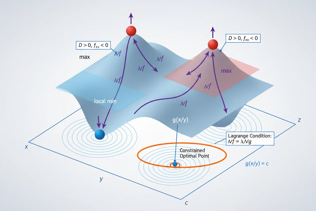
Optimization is the mathematical process of finding the largest or smallest possible value of a function under specified conditions. In calculus, optimization typically begins by identifying critical points where the derivative or gradient is zero or undefined, then determining whether those points represent maxima, minima, saddle points, or neither. For a one-variable function, candidates commonly satisfy f′(x) = 0, while a differentiable multivariable function typically requires ∇f = 0 at an unconstrained interior optimum. Boundary points and domain restrictions must also be checked because an absolute optimum does not have to occur at an interior critical point. Second derivatives, sign changes, curvature, and direct function-value comparisons can classify candidates. Constrained optimization adds relationships that the variables must satisfy and may use substitution or gradient-based methods. The central principle is not simply to solve a derivative equation, but to identify every legitimate candidate and compare them according to the domain and the type of optimum requested.
What Is Optimization?
Optimization asks questions such as:
What input produces the greatest output?
or:
What input produces the smallest output?
If:
y = f(x)
then a maximum occurs where f takes a value at least as large as nearby or permitted values, while a minimum occurs where it takes a value at least as small.
The broad topic includes both one-variable and multivariable calculus problems.
Typical applications include minimizing cost, maximizing profit, minimizing distance, maximizing area, finding efficient dimensions, locating extreme temperatures, and choosing the best combination of several variables.
Optimization Formula in One Variable
For a differentiable one-variable function:
y = f(x)
interior optimization candidates commonly satisfy:
f′(x) = 0
Such points are called stationary points.
Critical points also include domain points where:
f′(x)
does not exist.
Finding a critical point does not automatically prove that it is a maximum or minimum. Classification is still required.
The ordinary derivative supplies the local rate of change used in this calculation.
Optimization Formula in Several Variables
For:
z = f(x, y)
an interior differentiable optimum commonly satisfies:
∇f = 0
Since:
∇f = (fₓ, fᵧ)
this means solving:
fₓ = 0
and:
fᵧ = 0
simultaneously.
For three variables:
f(x, y, z)
the first-order condition becomes:
fₓ = 0
fᵧ = 0
f_z = 0
The individual components are partial derivative calculations.
Local Maximum
A point x = a is a local maximum if f(a) is at least as large as nearby function values.
Informally:
f(a) ≥ f(x)
for x sufficiently close to a.
For example:
f(x) = −x² + 4
has:
f′(x) = −2x
Set:
−2x = 0
so:
x = 0
The function value is:
f(0) = 4
Because the parabola opens downward, this point is both a local and global maximum.
Local Minimum
A point x = a is a local minimum if f(a) is no greater than nearby values.
Consider:
f(x) = x² + 3
Then:
f′(x) = 2x
Set:
2x = 0
so:
x = 0
The value is:
f(0) = 3
Because:
x² ≥ 0
for every real x:
f(x) ≥ 3
Therefore x = 0 gives both a local and absolute minimum.
Absolute Maximum and Minimum
A local optimum only compares the function with nearby points.
An absolute, or global, optimum compares it with every point in the permitted domain.
For example, a function may have several local peaks while only one is the highest overall.
A correct optimization solution must determine whether the question asks for:
local maximum
local minimum
absolute maximum
or:
absolute minimum
The domain is essential when finding global extrema.
Critical Points
A critical point of a one-variable function occurs at a domain value c where:
f′(c) = 0
or:
f′(c)
does not exist.
For example:
f(x) = |x|
has no derivative at:
x = 0
yet zero is an absolute minimum.
Therefore an optimization method that checks only:
f′(x) = 0
can miss valid extrema.
First Derivative Test
The first derivative test classifies a critical point by checking whether f′ changes sign.
If:
f′ changes from positive to negative
then f changes from increasing to decreasing, giving a local maximum.
If:
f′ changes from negative to positive
then f changes from decreasing to increasing, giving a local minimum.
If the sign does not change, the critical point is not a local extremum.
This test uses the behavior of derivatives around the candidate rather than just the derivative value at one point.
First Derivative Test Example
Consider:
f(x) = x³ − 3x
Differentiate:
f′(x) = 3x² − 3
Factor:
f′(x) = 3(x − 1)(x + 1)
Critical points are:
x = −1
and:
x = 1
For x < −1:
f′(x) > 0
Between −1 and 1:
f′(x) < 0
For x > 1:
f′(x) > 0
Therefore at:
x = −1
the derivative changes positive to negative, so there is a local maximum.
At:
x = 1
it changes negative to positive, so there is a local minimum.
Function values are:
f(−1) = 2
f(1) = −2
Second Derivative Test
If:
f′(c) = 0
and the second derivative exists, then:
f″(c) > 0 → local minimum
f″(c) < 0 → local maximum
If:
f″(c) = 0
the test is inconclusive.
A positive second derivative indicates local concave-up behavior. A negative second derivative indicates local concave-down behavior.
Second Derivative Example
Let:
f(x) = x² − 6x + 11
Differentiate:
f′(x) = 2x − 6
Set:
2x − 6 = 0
giving:
x = 3
Now:
f″(x) = 2
Therefore:
f″(3) = 2 > 0
so:
x = 3
is a local minimum.
Evaluate:
f(3) = 9 − 18 + 11
= 2
Thus the minimum point is:
(3, 2)
When the Second Derivative Test Fails
Consider:
f(x) = x⁴
At:
x = 0
we have:
f′(0) = 0
and:
f″(0) = 0
The second derivative test is inconclusive.
However:
x⁴ ≥ 0
for every real x.
Therefore:
x = 0
is an absolute minimum.
An inconclusive test does not mean no extremum exists. It means another method is needed.
Closed Interval Optimization
If a function is continuous on a closed interval:
[a, b]
an absolute maximum and minimum exist.
A practical procedure is:
- Find critical points inside (a, b).
- Evaluate f at every critical point.
- Evaluate f(a) and f(b).
- Compare all values.
The largest is the absolute maximum.
The smallest is the absolute minimum.
This procedure depends on the relationship between optimization and continuity.
Closed Interval Example
Find the absolute extrema of:
f(x) = x³ − 3x
on:
[−2, 2]
We already know:
f′(x) = 3(x² − 1)
so the critical points are:
x = −1
and:
x = 1
Evaluate all candidates.
At x = −2:
f(−2) = −8 + 6 = −2
Also, At x = −1:
f(−1) = 2
At x = 1:
f(1) = −2
At x = 2:
f(2) = 8 − 6 = 2
Therefore:
absolute maximum = 2
occurring at:
x = −1 and x = 2
and:
absolute minimum = −2
occurring at:
x = −2 and x = 1
Optimization From a Word Problem
Optimization problems often begin with several physical quantities rather than an explicit function f(x).
The essential steps are to identify the quantity being optimized, write it as a function, incorporate constraints, determine the valid domain, and then analyze extrema.
Consider a rectangle with perimeter:
40
Let its length be x and width be y.
Then:
2x + 2y = 40
so:
x + y = 20
and:
y = 20 − x
The area is:
A = xy
Substitute:
A(x) = x(20 − x)
= 20x − x²
Now the original two-variable geometry problem has become a one-variable optimization problem.
Maximum Rectangle Area
Differentiate:
A′(x) = 20 − 2x
Set:
A′(x) = 0
Then:
20 − 2x = 0
x = 10
Therefore:
y = 20 − 10 = 10
The second derivative is:
A″(x) = −2
Since it is negative:
x = 10
gives a maximum.
The maximum-area rectangle with perimeter 40 is therefore:
10 × 10
and its area is:
100
The optimal rectangle is a square.
Minimizing a Sum
Find two positive numbers whose sum is 20 and whose product is as large as possible.
Let:
x + y = 20
so:
y = 20 − x
The product is:
P(x) = x(20 − x)
This is exactly the same function:
P(x) = 20x − x²
Therefore the maximum occurs at:
x = 10
and:
y = 10
Different word problems can reduce to the same optimization structure.
Distance Optimization
The squared distance between:
(x, y)
and a fixed point:
(a, b)
is:
D² = (x − a)² + (y − b)²
When minimizing distance, it is often easier to minimize D² instead of:
D = √[(x − a)² + (y − b)²]
because the square-root function is increasing for nonnegative inputs.
The point minimizing D² also minimizes D.
Removing the square root can make derivatives significantly simpler.
Multivariable Optimization
For:
f(x, y)
calculate:
fₓ
and:
fᵧ
Then solve:
fₓ = 0
fᵧ = 0
These equations locate interior stationary points where:
∇f = 0
The gradient summarizes the first-order conditions in one vector equation.
Each candidate must then be classified.
Multivariable Example
Find the minimum of:
f(x, y) = x² + y² − 4x + 6y + 20
Calculate:
fₓ = 2x − 4
fᵧ = 2y + 6
Set both equal to zero:
2x − 4 = 0
so:
x = 2
and:
2y + 6 = 0
so:
y = −3
Complete the square:
f(x, y) = (x − 2)² + (y + 3)² + 7
Therefore the absolute minimum occurs at:
(2, −3)
with:
f(2, −3) = 7
Saddle Point
A critical point can be neither a maximum nor a minimum.
Consider:
f(x, y) = x² − y²
The partial derivatives are:
fₓ = 2x
fᵧ = −2y
Both vanish at:
(0, 0)
However, along:
y = 0
the function becomes:
f(x, 0) = x² ≥ 0
while along:
x = 0
it becomes:
f(0, y) = −y² ≤ 0
The function rises in one direction and falls in another.
Therefore:
(0, 0)
is a saddle point.
Second Derivative Test in Two Variables
For:
f(x, y)
define:
D = fₓₓfᵧᵧ − (fₓᵧ)²
at a critical point.
Then:
D > 0 and fₓₓ > 0 → local minimum
D > 0 and fₓₓ < 0 → local maximum
D < 0 → saddle point
D = 0 → inconclusive
This determinant measures second-order curvature behavior.
Two-Variable Classification Example
Consider:
f(x, y) = x² + 4y²
The only critical point is:
(0, 0)
Second partial derivatives are:
fₓₓ = 2
fᵧᵧ = 8
fₓᵧ = 0
Therefore:
D = 2(8) − 0²
= 16
Since:
D > 0
and:
fₓₓ > 0
the point:
(0, 0)
is a local minimum.
In fact, because the function is nonnegative everywhere, it is the global minimum.
Hessian Matrix
Second partial derivatives can be organized into the Hessian matrix:
H = [ fₓₓ fₓᵧ ]
[ fᵧₓ fᵧᵧ ]
for a two-variable function.
For sufficiently smooth functions:
fₓᵧ = fᵧₓ
The Hessian describes local second-order curvature.
Properties involving eigenvalues, determinants, and matrix operations provide a systematic way to classify multidimensional critical points.
The detailed matrix algebra supports rather than replaces the calculus conditions.
Hessian and Matrix Rank
The matrix rank of derivative or constraint matrices can become important when an optimization problem contains several interacting variables or constraints.
Rank tells us how many independent first-order conditions are actually present.
If supposedly different constraints have dependent gradients, the effective number of independent restrictions is smaller than the number of equations written.
This becomes especially important in constrained multivariable problems.
Direction of Steepest Descent
If:
∇f ≠ 0
then the direction of steepest local increase is:
∇f/|∇f|
The direction of steepest local decrease is:
−∇f/|∇f|
This follows from the directional derivative formula:
Dᵤf = ∇f · u
For a unit vector u, the most negative value occurs when u points opposite the gradient.
This is the geometric principle behind gradient-descent methods.
Gradient Descent Update
A basic iterative optimization update is:
xₙ₊₁ = xₙ − α∇f(xₙ)
where:
α > 0
is the step size.
The negative gradient supplies a local descent direction.
A small enough step often decreases the objective locally, but choosing α appropriately matters.
A step that is too large can overshoot or even cause divergence.
Gradient descent is a numerical optimization method rather than a replacement for exact critical-point analysis.
One-Dimensional Descent Example
Suppose:
f(x) = x²
Then:
f′(x) = 2x
A gradient-style update becomes:
xₙ₊₁ = xₙ − α(2xₙ)
If:
α = 0.1
then:
xₙ₊₁ = 0.8xₙ
Starting from:
x₀ = 10
gives:
x₁ = 8
x₂ = 6.4
x₃ = 5.12
The sequence moves toward the minimum:
x = 0
Constrained Optimization
A constrained optimization problem restricts the permissible inputs.
For example:
maximize f(x, y)
subject to:
g(x, y) = c
The optimum must lie on the constraint rather than anywhere in the full plane.
Sometimes the constraint can be solved directly for one variable and substituted into the objective.
When that is inconvenient, a gradient-based constrained method can be used.
Constraint by Substitution
Suppose we want to maximize:
f(x, y) = xy
subject to:
x + y = 20
Solve:
y = 20 − x
Then:
f(x) = x(20 − x)
The multivariable constrained problem reduces to the one-variable problem already solved.
The maximum occurs at:
x = 10
y = 10
Substitution is often the simplest constrained method when the constraint isolates easily.
Lagrange Multiplier Condition
For a regular constraint:
g(x, y) = c
a candidate constrained optimum can satisfy:
∇f = λ∇g
together with:
g(x, y) = c
The scalar λ is called a Lagrange multiplier.
Geometrically, at a regular constrained extremum the level curve of f is tangent to the constraint, so their gradients are parallel.
Lagrange Multiplier Example
Maximize:
f(x, y) = xy
subject to:
x + y = 20
Let:
g(x, y) = x + y
Then:
∇f = (y, x)
and:
∇g = (1, 1)
Set:
(y, x) = λ(1, 1)
Therefore:
y = λ
x = λ
so:
x = y
Use the constraint:
x + y = 20
giving:
2x = 20
x = 10
and:
y = 10
The product is:
100
This agrees with the substitution method.
Boundary Optimization in Several Variables
A closed two-dimensional region can have extrema:
- at interior critical points,
- on boundary curves,
- or at boundary corners/endpoints.
Checking only:
∇f = 0
is therefore insufficient for an absolute optimization problem on a bounded region.
The boundary must be converted into one or more lower-dimensional optimization problems and checked separately.
This is the multivariable analogue of checking endpoints on a closed interval.
Optimization and Implicit Constraints
Constraints are frequently given implicitly:
F(x, y) = 0
The geometry of the constraint can be understood using implicit differentiation or gradients.
For a smooth constraint:
∇F
is normal to the constraint curve.
At a constrained optimum, the objective gradient may align with this normal direction.
This explains geometrically why gradient-based constrained methods work.
Optimization and Linear Approximation
A linear approximation predicts local change:
Δf ≈ ∇f · Δx
If:
∇f ≠ 0
there is a direction in which the first-order approximation decreases.
At an unconstrained interior differentiable minimum or maximum:
∇f = 0
so the first-order linear term vanishes.
Second-order behavior then becomes important for classification.
Optimization and Differentials
In one variable:
dy = f′(x)dx
In several variables:
df = fₓdx + fᵧdy
The differentials expression gives first-order output change.
At an unconstrained stationary point:
fₓ = fᵧ = 0
so:
df = 0
for every first-order displacement.
This is another way to express the vanishing-gradient condition.
Optimization and the Chain Rule
The chain rule is important when an objective is expressed through other changing quantities.
Suppose:
z = f(x, y)
and both x and y depend on t.
Then:
dz/dt = fₓ dx/dt + fᵧ dy/dt
An optimization problem along a parameterized path can use this derivative to find points where the objective stops increasing or decreasing along that path.
Optimization and Limits
Optimization relies on local behavior, which is ultimately grounded in limits.
Derivatives are defined through limits, and derivative sign changes identify rising and falling behavior.
In theoretical settings, existence of extrema also depends on continuity and domain properties.
The singular limit calculation itself is therefore not an optimization method, but it supplies part of the foundation for the derivative tests optimization uses.
Optimization and Integration
Some objective functions are defined by accumulated quantities.
For example:
F(x) = ∫₀ˣ f(t)dt
Then the Fundamental Theorem Of Calculus may give:
F′(x) = f(x)
An optimization problem for F can therefore reduce to finding where:
f(x) = 0
and analyzing sign changes.
Integration may construct the objective, while differentiation locates its extrema.
Optimization and Partial Fraction Integration
Partial fraction integration solves rational integration problems and is not itself an optimization technique.
The two can nevertheless appear in the same calculation if an objective function is defined through an accumulated rational expression that must first be integrated.
Once the objective is available, optimization still requires derivative, domain, boundary, and classification analysis.
Keeping these stages separate avoids confusing integration technique with extremum testing.
Optimization and Matrix Structure
For higher-dimensional objectives, derivative and curvature information can be stored in vectors and matrices.
The gradient records first-order rates.
The Hessian records second-order rates.
A positive-definite Hessian at a stationary point supports a local minimum; a negative-definite Hessian supports a local maximum; an indefinite Hessian supports a saddle point.
Eigenvalues can help determine these matrix properties.
This is where calculus and linear algebra interact strongly within Calculus & Linear Algebra.
Optimization With Domain Restrictions
An algebraic critical point is irrelevant if it lies outside the permitted domain.
Suppose a variable represents length.
Then:
x > 0
may be required.
A derivative equation might produce negative candidates, but those values must be discarded if they violate the physical or mathematical constraints.
Likewise, denominator restrictions, square roots, logarithms, and geometry can impose domain boundaries that need separate evaluation.
Optimization With Discrete Restrictions
Calculus optimization assumes variables can usually vary continuously.
If an application requires:
x must be an integer
the continuous optimum can still provide useful guidance, but nearby permissible integers must be compared.
For example, if the continuous optimum is:
x = 6.4
and only whole numbers are valid, likely candidates include:
x = 6
and:
x = 7
The final choice must respect the actual feasible set.
Optimization and Units
Units can reveal setup errors.
If the objective is area:
A = xy
and x and y are measured in meters, then A has units:
m²
If a constraint is perimeter, its terms must have units:
m
Differentiating an objective changes units accordingly.
For example:
dA/dx
has units of area per unit length:
m²/m = m
Dimensional consistency is a practical check before solving an optimization model.
Common Optimization Mistakes
A common mistake is setting the derivative equal to zero and stopping. A critical point is only a candidate.
Another error is forgetting points where the derivative does not exist.
Absolute extrema on closed intervals require endpoint checks.
Multivariable absolute extrema on bounded regions require boundary analysis.
A zero gradient does not automatically imply a minimum; saddle points can also satisfy:
∇f = 0
The second derivative test may be inconclusive and should not be forced into a classification when its determinant or second derivative vanishes.
Domain restrictions must be applied before accepting a candidate.
Finally, the objective function should be written in as few independent variables as the constraints allow. Differentiating before using the constraint often produces unnecessary complexity.
Frequently Asked Questions
What is optimization in calculus?
Optimization is the process of finding maximum or minimum values of a function subject to its domain and any additional constraints.
What is the basic optimization condition in one variable?
For an interior differentiable optimum, a common necessary condition is:
f′(x) = 0
Critical points where f′ does not exist must also be considered.
What is the optimization condition in several variables?
For an unconstrained interior differentiable optimum:
∇f = 0
which means all first partial derivatives equal zero.
Does f′(x) = 0 guarantee a maximum or minimum?
No. It identifies a stationary candidate. The point may be a maximum, minimum, saddle-type point in several variables, or neither.
What is the first derivative test?
It classifies a critical point by checking how the sign of f′ changes across the point.
What is the second derivative test in one variable?
If f′(c) = 0:
f″(c) > 0 → local minimum
f″(c) < 0 → local maximum
f″(c) = 0 → inconclusive
What should be checked on a closed interval?
Evaluate the function at all interior critical points and both endpoints, then compare the values.
How do you optimize with a constraint?
If possible, solve the constraint for one variable and substitute it into the objective. More complex smooth equality constraints can use gradient-based methods such as Lagrange multipliers.
What is a saddle point?
It is a critical point where the function increases in some directions and decreases in others, so it is neither a local maximum nor minimum.
What direction decreases a function fastest?
When ∇f ≠ 0, the unit direction of steepest local decrease is:
−∇f/|∇f|
Why are boundaries important in optimization?
An absolute maximum or minimum can occur on a boundary even when there is no interior critical point there.
How can I check an optimization answer?
Verify the candidate satisfies the domain and constraints, classify it correctly, evaluate all required boundary or endpoint candidates, and compare function values when an absolute extremum is requested.




