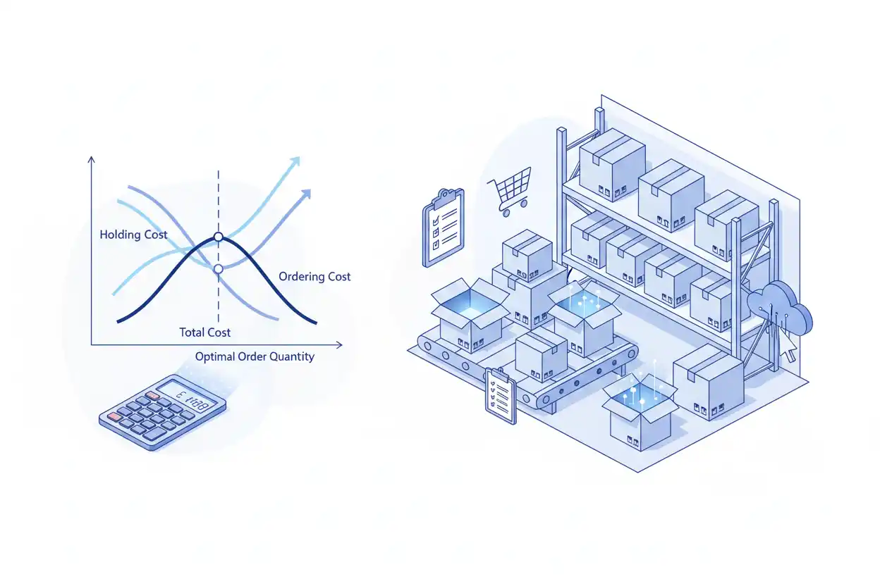
Economic order quantity, or EOQ, is the order size that minimizes the combined annual ordering and inventory holding costs under the standard EOQ model assumptions.
The formula balances two competing effects. Ordering larger quantities reduces how often a business places orders, lowering ordering cost, but it increases average inventory and therefore raises holding cost. Smaller orders do the opposite.
EOQ identifies the point where those two cost pressures are balanced.
What Is Economic Order Quantity?
Economic order quantity answers a specific inventory decision:
How many units should the business order each time?
It does not determine when the order should be placed. That is a separate question handled by the reorder point.
It also does not determine how much buffer inventory should be carried for uncertainty. That is the role of safety stock.
EOQ focuses on the order quantity that minimizes relevant ordering and holding costs under a simplified set of conditions.
Economic Order Quantity Formula
The classic EOQ formula is:
EOQ = √((2 × D × S) ÷ H)
Where:
D = annual demand in units
S = ordering cost per order
H = annual holding cost per unit
The result is the theoretically optimal number of units to order each time.
The units must be consistent. If demand is annual, the holding cost should also be expressed on an annual per-unit basis.
Economic Order Quantity Example
Suppose a retailer expects:
- annual demand of 10,000 units;
- ordering cost of $50 per order; and
- annual holding cost of $2 per unit.
Insert the values:
EOQ = √((2 × 10,000 × $50) ÷ $2)
First calculate the numerator:
2 × 10,000 × 50 = 1,000,000
Divide by holding cost:
1,000,000 ÷ 2 = 500,000
Take the square root:
EOQ = √500,000 ≈ 707.11 units
The theoretical economic order quantity is approximately 707 units per order.
A business would normally round to a practical whole-unit or supplier-compatible quantity.
Verify the EOQ Result
At an EOQ of approximately 707.11 units, the annual number of orders is:
Annual Orders = Annual Demand ÷ EOQ
Annual Orders = 10,000 ÷ 707.11 ≈ 14.14 orders
Average cycle inventory under the standard EOQ assumptions is:
Average Inventory = EOQ ÷ 2
Average Inventory = 707.11 ÷ 2 ≈ 353.55 units
Annual ordering cost is:
Ordering Cost = (D ÷ Q) × S
Ordering Cost = (10,000 ÷ 707.11) × $50 ≈ $707.11
Annual holding cost is:
Holding Cost = (Q ÷ 2) × H
Holding Cost = (707.11 ÷ 2) × $2 ≈ $707.11
At the theoretical EOQ:
Annual Ordering Cost ≈ Annual Holding Cost
Both are approximately $707.11 in this example.
The combined relevant annual cost is:
$707.11 + $707.11 = $1,414.22
The slight rounding difference comes from rounding the EOQ result.
Why the EOQ Formula Works
Ordering cost falls as order quantity increases.
Suppose annual demand is 10,000 units.
If the business orders 100 units each time:
10,000 ÷ 100 = 100 orders per year
If it orders 1,000 units each time:
10,000 ÷ 1,000 = 10 orders per year
Fewer orders generally mean lower annual ordering costs.
However, larger orders create higher average inventory.
At an order quantity of 100 units:
Average Cycle Inventory = 100 ÷ 2 = 50 units
At 1,000 units:
Average Cycle Inventory = 1,000 ÷ 2 = 500 units
Higher average inventory creates more inventory carrying cost.
EOQ finds the point where reducing one cost further would increase the other enough to outweigh the saving.
Ordering Cost Formula
The annual ordering-cost component of the EOQ model is:
Annual Ordering Cost = (D ÷ Q) × S
Where:
D is annual demand.
Q is order quantity.
S is cost per order.
Suppose annual demand is 24,000 units, order size is 1,200 units, and ordering cost is $75.
The company places:
24,000 ÷ 1,200 = 20 orders
Annual ordering cost is:
20 × $75 = $1,500
Increasing the order size would reduce the number of annual orders, assuming demand remains unchanged.
Holding Cost Formula
Under the standard no-safety-stock EOQ model, average cycle inventory is:
Average Inventory = Q ÷ 2
Annual holding cost is therefore:
Annual Holding Cost = (Q ÷ 2) × H
Suppose the company orders 1,200 units at a time and annual holding cost is $3 per unit.
Average cycle inventory is:
1,200 ÷ 2 = 600 units
Annual holding cost is:
600 × $3 = $1,800
Increasing the order quantity therefore reduces ordering frequency but increases inventory held on average.
Total Relevant EOQ Cost
The two principal relevant costs can be combined:
Total Relevant Cost = (D ÷ Q) × S + (Q ÷ 2) × H
The EOQ formula identifies the value of Q that minimizes this relationship under the model assumptions.
Purchase cost is usually excluded from this optimization when the unit purchase price does not change with order quantity.
If quantity discounts alter purchase price, the basic EOQ result may no longer identify the lowest total-cost option by itself.
A Second EOQ Example
Suppose a company has:
- Annual demand: 24,000 units
- Ordering cost: $75 per order
- Annual holding cost: $3 per unit
Calculate:
EOQ = √((2 × 24,000 × 75) ÷ 3)
Multiply:
2 × 24,000 × 75 = 3,600,000
Divide:
3,600,000 ÷ 3 = 1,200,000
Take the square root:
EOQ = √1,200,000 ≈ 1,095.45 units
The theoretical order quantity is approximately 1,095 units.
Annual orders:
24,000 ÷ 1,095.45 ≈ 21.91 orders
Average cycle inventory:
1,095.45 ÷ 2 ≈ 547.72 units
Annual ordering cost:
21.91 × $75 ≈ $1,643.17
Annual holding cost:
547.72 × $3 ≈ $1,643.17
Again, the two relevant costs are approximately equal at the EOQ.
EOQ vs. Reorder Point
EOQ and reorder point solve different inventory problems.
EOQ asks: How much should we order?
Reorder point asks: At what inventory level should we place the next order?
A company might calculate an EOQ of 700 units but determine that an order should be triggered whenever inventory falls to 250 units.
The calculations can work together, but the reorder point should remain separate from the EOQ quantity itself.
EOQ vs. Safety Stock
EOQ is also different from safety stock.
Safety stock is additional inventory held to protect against uncertainty such as unexpected demand or supplier delays.
The basic EOQ formula assumes stable conditions and does not include a safety-stock term.
If safety stock is held, average inventory may be approximated as:
Average Inventory ≈ EOQ ÷ 2 + Safety Stock
Suppose EOQ is 700 units and safety stock is 150 units:
Average Inventory ≈ 700 ÷ 2 + 150
Average Inventory ≈ 350 + 150 = 500 units
Safety stock raises inventory carried on average, but it does not automatically change the classic EOQ calculation unless the relevant cost assumptions themselves change.
EOQ and Inventory
Inventory ties up capital and can create storage, insurance, handling, shrinkage, obsolescence, and financing costs.
That makes ordering “as much as possible” economically inefficient even if larger purchases reduce ordering frequency.
At the other extreme, extremely small orders can create excessive purchasing, receiving, transportation, administrative, and setup costs.
EOQ provides a structured compromise between those extremes.
What Counts as Ordering Cost?
Ordering cost should represent costs that meaningfully change with the number of orders placed.
Depending on the business, relevant components can include purchase-order processing, receiving administration, setup costs, inspections, or other incremental costs caused by placing an order.
Suppose a company estimates:
- purchasing labor per order: $25;
- receiving administration: $15;
- inspection and processing: $10.
Then:
Ordering Cost per Order = $25 + $15 + $10 = $50
That $50 could be used as S if those costs genuinely behave as order-level costs.
Fixed costs that will be incurred regardless of order frequency should not automatically be forced into the ordering-cost estimate.
What Counts as Holding Cost?
Annual holding cost per unit can reflect relevant costs associated with carrying one additional unit of inventory for a year.
Possible components include storage, insurance, deterioration, shrinkage, obsolescence risk, and the opportunity cost of capital tied up in stock.
Suppose a product costs $40 and the company estimates an annual carrying-cost rate of 20%.
A simplified annual holding-cost estimate would be:
H = $40 × 20% = $8 per Unit per Year
That $8 could then be used in the EOQ model, provided the carrying-cost rate appropriately captures the relevant holding economics.
The detailed construction of these costs belongs to inventory carrying cost analysis rather than the EOQ formula itself.
EOQ When Holding Cost Is a Percentage
If annual holding cost is stated as a percentage of unit cost:
H = Unit Cost × Carrying Cost Rate
Suppose:
- Unit cost = $25
- Carrying-cost rate = 24%
Then:
H = $25 × 24% = $6 per Unit per Year
If annual demand is 18,000 units and ordering cost is $40:
EOQ = √((2 × 18,000 × 40) ÷ 6)
EOQ = √240,000 ≈ 489.90 units
A practical order size could therefore be approximately 490 units, subject to packaging, supplier, capacity, and operational constraints.
EOQ and Inventory Turnover
Inventory turnover measures how frequently inventory is sold or consumed relative to the inventory base.
EOQ addresses a different issue: the economically efficient replenishment quantity under specified assumptions.
A company can have a mathematically reasonable EOQ yet poor inventory turnover if demand forecasts are wrong, obsolete products accumulate, or stock is poorly managed.
Likewise, rapid inventory turnover does not prove that order quantities minimize ordering and carrying costs.
The metrics complement rather than replace each other.
EOQ and Cost of Goods Sold
Cost of goods sold measures the inventory cost associated with goods actually sold during a period.
EOQ determines a suggested replenishment quantity.
Ordering 700 units does not mean 700 units immediately become COGS.
Purchased items normally enter inventory first. Their costs become COGS when the related goods are sold under the applicable accounting treatment.
This distinction separates procurement decisions from financial-statement cost recognition.
EOQ and Double-Entry Bookkeeping
The EOQ model determines a suggested order size; double-entry bookkeeping records what happens financially when the business actually purchases inventory.
Suppose EOQ recommends ordering 700 units at $20 each.
The purchase value is:
700 × $20 = $14,000
If purchased on credit, the accounting system may record an increase in inventory and an increase in accounts payable.
The EOQ formula itself does not create a journal entry.
It is an operational decision model, while bookkeeping records the resulting transaction.
Debit and Credit Do Not Determine EOQ
Similarly, debit and credit rules determine how purchases and payments are recorded, not how many units should be ordered.
The business should not include bookkeeping mechanics as ordering-cost variables merely because entries are required when inventory is purchased.
Only costs that are economically relevant to order frequency belong in the EOQ assumptions.
Should Depreciation Expense Be Included in Holding Cost?
Depreciation expense should not automatically be included in EOQ holding cost.
Suppose a warehouse building depreciates by $100,000 annually regardless of whether average inventory is 5,000 or 6,000 units.
That fixed accounting depreciation does not necessarily represent an incremental cost of carrying one additional unit.
However, if additional inventory genuinely causes additional equipment use, storage infrastructure, or other incremental capacity costs, those economics may deserve consideration.
The EOQ model works best when H captures relevant incremental carrying costs rather than every accounting expense associated with inventory operations.
Demand Forecasts Matter
EOQ depends directly on annual demand D.
If the demand estimate is wrong, the calculated EOQ will also change.
Suppose expected annual demand is 10,000 units but actual demand becomes 14,400 units, with ordering cost of $50 and holding cost of $2.
Original EOQ:
EOQ = √((2 × 10,000 × 50) ÷ 2) ≈ 707 units
Revised EOQ:
EOQ = √((2 × 14,400 × 50) ÷ 2)
EOQ = √720,000 ≈ 849 units
Higher expected demand increases the optimal order quantity, but less than proportionally because demand is inside a square root.
EOQ and Forecast Variance
A forecast variance can reveal that actual demand differed materially from the demand assumption used in EOQ.
Suppose annual demand was forecast at 20,000 units but current evidence points toward 25,000.
The EOQ should be recalculated if that revised estimate is operationally meaningful.
Using stale demand inputs can produce precise-looking calculations that no longer represent current conditions.
Forecast accuracy therefore affects EOQ quality even though forecast variance remains a separate analytical measure.
EOQ Sensitivity to Ordering Cost
Suppose annual demand is 10,000 units and annual holding cost is $2 per unit.
At an ordering cost of $50:
EOQ ≈ 707 units
If ordering cost falls to $20 because purchasing becomes more automated:
EOQ = √((2 × 10,000 × 20) ÷ 2)
EOQ = √200,000 ≈ 447 units
Lower ordering cost makes smaller, more frequent orders economically attractive.
This is why process automation can change the appropriate replenishment quantity.
EOQ Sensitivity to Holding Cost
Now assume annual demand remains 10,000 units and ordering cost remains $50.
At $2 annual holding cost:
EOQ ≈ 707 units
If annual holding cost rises to $8 per unit:
EOQ = √((2 × 10,000 × 50) ÷ 8)
EOQ = √125,000 ≈ 354 units
Higher holding cost pushes the optimal order quantity lower because carrying large quantities becomes more expensive.
Does EOQ Minimize All Inventory Costs?
No.
The classic EOQ model minimizes the combination of ordering and holding costs under its assumptions.
It does not automatically minimize:
- stockout costs;
- purchase prices that vary by quantity;
- capacity constraints;
- spoilage under irregular demand;
- supplier-risk costs;
- transportation constraints; or
- every broader business expense.
The output should therefore be treated as a decision model rather than an unquestionable purchasing rule.
EOQ Assumptions
The classic EOQ formula relies on simplifying assumptions.
Demand is generally assumed to be known and reasonably constant.
Ordering cost per order and holding cost per unit are treated as stable.
Replenishment is assumed to occur predictably.
The basic model also assumes no quantity discounts and typically excludes stockouts from the optimization.
Real businesses often violate some of these assumptions.
EOQ can still provide a useful baseline, but the more the operating environment differs from the model, the more adjustment and judgment are required.
Quantity Discounts Can Change the Decision
Suppose the calculated EOQ is 700 units, but a supplier offers a lower unit price for orders of at least 1,000 units.
Ordering 1,000 units increases average inventory and holding costs, but the purchase-price saving may outweigh that increase.
The decision then requires comparing total relevant costs at feasible order quantities.
The basic EOQ value should not be accepted automatically when purchase prices change with quantity.
Minimum Order Quantities
A supplier may require a minimum order quantity greater than the calculated EOQ.
Suppose:
Calculated EOQ = 600 units
but:
Supplier Minimum = 1,000 units
The company cannot practically order 600 units under that supplier agreement.
EOQ remains useful as a benchmark because it shows that the supplier constraint is forcing the business above the theoretical cost-minimizing quantity.
Management can then evaluate alternative suppliers, negotiate terms, or accept the higher carrying cost.
Pack Sizes and Whole Units
EOQ often produces a decimal result such as 707.11 units.
A business cannot order 0.11 of a packaged product.
If products are shipped in cases of 24 units, the nearest practical quantities might be:
696 units = 29 cases
or:
720 units = 30 cases
Because the total-cost curve is relatively flat near its minimum in many EOQ situations, a nearby practical quantity can often have little cost difference from the exact mathematical result.
The practical alternatives should still be checked when the financial stakes are material.
EOQ and Gross Burn
Gross burn measures cash spending in a different analytical context. It should not be substituted for EOQ holding or ordering costs.
Large inventory purchases can affect cash outflows and therefore liquidity, but EOQ focuses on minimizing relevant inventory ordering and carrying costs.
A company could have an economically reasonable EOQ and still face cash constraints that make the recommended purchase difficult to finance.
Inventory optimization and cash-burn analysis therefore need to remain distinct.
When EOQ Is Most Useful
EOQ tends to be most informative when demand is reasonably predictable, replenishment economics are stable, the product is repeatedly ordered, and ordering and holding costs can be estimated meaningfully.
It can be less reliable for highly seasonal products, fashion inventory, short-life products, uncertain supply chains, rapidly changing demand, or items with complex quantity discounts.
In those environments, EOQ can still serve as a baseline rather than a complete inventory policy.
Common Economic Order Quantity Mistakes
A common mistake is confusing EOQ with reorder point. EOQ determines how much to order; reorder point determines when to order.
Another error is using monthly demand with annual holding cost without converting the units to the same time basis.
Businesses may also underestimate holding cost by considering warehouse rent while ignoring capital, insurance, shrinkage, or obsolescence where relevant.
Another mistake is including fixed costs that do not change with order frequency.
Using a stale demand estimate can also make the answer misleading.
Finally, a precise EOQ result should not override supplier pack sizes, minimum orders, capacity constraints, cash limitations, or other real operating conditions.
Frequently Asked Questions
What is economic order quantity in simple terms?
Economic order quantity is the order size that minimizes the combined ordering and holding costs under the classic EOQ assumptions.
What is the EOQ formula?
The standard formula is:
EOQ = √((2 × D × S) ÷ H)
Where D is annual demand, S is ordering cost per order, and H is annual holding cost per unit.
What does an EOQ of 700 mean?
It means the model estimates that ordering approximately 700 units each time minimizes the relevant annual ordering and holding costs under the assumptions used.
It does not mean the company should always keep 700 units in inventory.
Is EOQ the same as reorder point?
No.
EOQ determines how much to order.
Reorder point determines when to place the order.
Does EOQ include safety stock?
The classic EOQ formula does not directly include safety stock.
Safety stock may be added when estimating total average inventory, but it serves a different purpose: protecting against uncertainty.
Why are ordering cost and holding cost equal at EOQ?
Under the standard EOQ model, the mathematical minimum occurs where annual ordering cost equals annual holding cost.
This equality provides a useful check on the calculated EOQ.
Does EOQ include purchase cost?
The classic formula does not need purchase cost when unit price remains constant regardless of order size.
Purchase cost becomes important when quantity discounts or other pricing changes exist.
What happens if demand increases?
All else equal, EOQ increases.
Because demand appears inside a square root, EOQ rises more slowly than demand itself.
What happens if holding cost increases?
EOQ decreases.
Higher holding costs make smaller, more frequent orders relatively attractive.
What happens if ordering cost decreases?
EOQ decreases.
When placing an order becomes cheaper, the business can order smaller quantities more frequently without incurring as much ordering expense.
Can EOQ be a decimal?
Yes mathematically.
In practice, the result is usually adjusted to whole units, case quantities, pallets, supplier minimums, or other feasible order sizes.
Is EOQ always the best order quantity?
No.
EOQ is optimal only within the assumptions of the model. Quantity discounts, uncertain demand, stockout risk, perishability, supplier constraints, cash limits, and capacity issues can justify a different quantity.
Used with those limits understood, economic order quantity is a valuable tool within broader accounting and operations planning.