


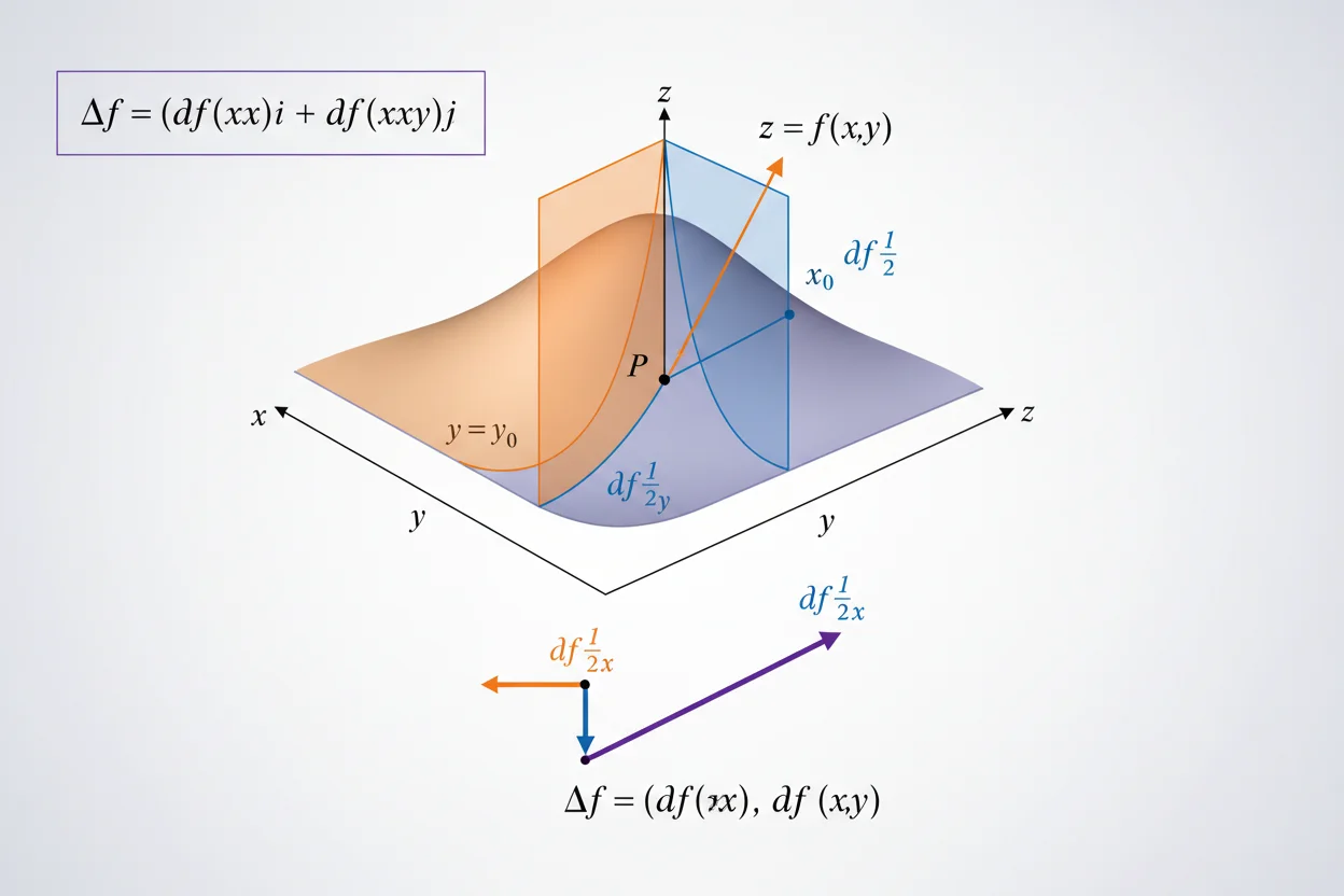
A partial derivative measures how a multivariable function changes with respect to one input variable while the other independent variables are held constant. For a function f(x, y), the two first partial derivatives are ∂f/∂x and ∂f/∂y. To calculate ∂f/∂x, differentiate with respect to x exactly as in ordinary calculus while treating y as a constant; to calculate ∂f/∂y, reverse those roles. For example, if f(x, y) = x²y + 3y², then ∂f/∂x = 2xy and ∂f/∂y = x² + 6y. Partial derivatives describe slopes along coordinate directions and form the components of the gradient. They also support tangent planes, linear approximation, multivariable chain rules, optimization, differential equations, and derivative matrices. Higher-order partial derivatives measure repeated and mixed changes, such as ∂²f/∂x² and ∂²f/∂y∂x. The central calculation rule is simple: identify the differentiation variable and temporarily treat the other independent variables as constants.
What Is a Partial Derivative?
A one-variable function:
y = f(x)
has one independent input direction, so an ordinary derivative measures change with respect to x.
A multivariable function:
z = f(x, y)
has at least two independent input directions.
The partial derivative:
∂f/∂x
measures the rate of change as x varies while y is held constant.
Similarly:
∂f/∂y
measures the rate of change as y varies while x is held constant.
This is one of the foundational ideas of multivariable calculus.
Partial Derivative Notation
Common notation includes:
∂f/∂x
fₓ
Dₓf
for the partial derivative with respect to x.
With respect to y:
∂f/∂y
fᵧ
Dᵧf
The symbol:
∂
distinguishes partial differentiation from the ordinary derivative notation:
d/dx
used when a function depends on one independent variable.
Partial Derivative Formula
The partial derivative with respect to x can be defined by a limit:
∂f/∂x (a, b) = lim [f(a+h, b) − f(a, b)]/h as h → 0
Similarly:
∂f/∂y (a, b) = lim [f(a, b+h) − f(a, b)]/h as h → 0
The first formula changes x while fixing y = b.
The second changes y while fixing x = a.
These definitions connect partial derivatives directly with the ordinary limit definition of a derivative.
Basic Partial Derivative Example
Let:
f(x, y) = x²y + 3y²
Find:
fₓ
Treat y as constant.
Differentiate:
x²y → 2xy
and:
3y² → 0
Therefore:
fₓ = 2xy
Now find:
fᵧ
Treat x as constant.
Differentiate:
x²y → x²
and:
3y² → 6y
Therefore:
fᵧ = x² + 6y
Evaluate Partial Derivatives at a Point
For:
f(x, y) = x²y + 3y²
we found:
fₓ = 2xy
fᵧ = x² + 6y
At:
(2, 1)
we obtain:
fₓ(2, 1) = 2(2)(1)
= 4
and:
fᵧ(2, 1) = 2² + 6(1)
= 4 + 6
= 10
So at that point, the rate in the positive x-direction is 4, while the rate in the positive y-direction is 10.
Holding Other Variables Constant
Consider:
f(x, y) = 4x³y²
To differentiate with respect to x, treat:
4y²
as a constant coefficient.
Therefore:
fₓ = 12x²y²
To differentiate with respect to y, treat:
4x³
as constant.
Therefore:
fᵧ = 8x³y
The function itself is the same, but the active differentiation variable determines which factors change.
Power Rule for Partial Derivatives
The ordinary power rule still applies.
For example:
f(x, y) = x⁵y³
With respect to x:
fₓ = 5x⁴y³
With respect to y:
fᵧ = 3x⁵y²
The unaffected variable simply behaves as a multiplicative constant during each calculation.
Polynomial Example
Let:
f(x, y) = 3x⁴ − 5x²y + 7xy³ − 2y⁴
Differentiate with respect to x:
fₓ = 12x³ − 10xy + 7y³
because:
−2y⁴
is constant relative to x.
Differentiate with respect to y:
fᵧ = −5x² + 21xy² − 8y³
because:
3x⁴
is constant relative to y.
Partial Derivative With Three Variables
Suppose:
f(x, y, z) = x²y + yz³ + 4xz
There are three first partial derivatives.
With respect to x:
fₓ = 2xy + 4z
Also, With respect to y:
fᵧ = x² + z³
With respect to z:
f_z = 3yz² + 4x
Each time, the other two independent variables are held constant.
Product Rule With Partial Derivatives
The ordinary product rule remains valid.
Suppose:
f(x, y) = x²e^(xy)
Find fₓ.
Treat y as constant, but both:
x²
and:
e^(xy)
depend on x.
Apply the product rule:
fₓ = 2x e^(xy) + x²e^(xy)y
Therefore:
fₓ = e^(xy)(2x + x²y)
The ordinary product rule is applied with respect to the selected variable.
Find fᵧ for the Same Function
For:
f(x, y) = x²e^(xy)
treat x² as constant while differentiating with respect to y.
Using the chain rule:
d/dy[e^(xy)] = xe^(xy)
Therefore:
fᵧ = x² · xe^(xy)
= x³e^(xy)
The same expression can produce very different-looking partial derivatives.
Chain Rule Inside Partial Differentiation
Consider:
f(x, y) = sin(x² + y³)
For the x-partial:
fₓ = cos(x² + y³)(2x)
Therefore:
fₓ = 2x cos(x² + y³)
For the y-partial:
fᵧ = cos(x² + y³)(3y²)
Therefore:
fᵧ = 3y² cos(x² + y³)
The ordinary chain rule applies separately with respect to the chosen variable.
Quotient Rule Example
Let:
f(x, y) = x/(x + y)
Find fₓ.
Treat y as constant.
Using the quotient rule:
fₓ = [(x + y)(1) − x(1)]/(x + y)²
Simplify:
fₓ = y/(x + y)²
Now differentiate with respect to y.
Treat x as constant:
fᵧ = [0(x + y) − x(1)]/(x + y)²
Therefore:
fᵧ = −x/(x + y)²
where:
x + y ≠ 0
Exponential Partial Derivatives
Suppose:
f(x, y) = e^(2x+3y)
Then:
fₓ = 2e^(2x+3y)
because the derivative of:
2x + 3y
with respect to x is:
2
Similarly:
fᵧ = 3e^(2x+3y)
The same chain-rule structure appears in each coordinate direction.
Logarithmic Partial Derivatives
Let:
f(x, y) = ln(x² + y²)
For:
x² + y² > 0
the partial derivative with respect to x is:
fₓ = 2x/(x² + y²)
The partial derivative with respect to y is:
fᵧ = 2y/(x² + y²)
The point:
(0, 0)
is excluded because the logarithm argument becomes zero.
Domain restrictions therefore matter in partial differentiation just as they do in ordinary calculus.
Trigonometric Example
Consider:
f(x, y) = x sin y + y cos x
With respect to x:
fₓ = sin y − y sin x
With respect to y:
fᵧ = x cos y + cos x
Each term must be examined according to whether the selected differentiation variable occurs within it.
Geometric Meaning
For a surface:
z = f(x, y)
the partial derivative:
fₓ(a, b)
is the slope of the curve obtained by intersecting the surface with the vertical plane:
y = b
Similarly:
fᵧ(a, b)
is the slope of the slice:
x = a
So partial derivatives describe tangent slopes along coordinate-aligned slices of a surface.
They do not by themselves describe every possible directional slope.
Partial Derivatives and the Gradient
The gradient collects all first partial derivatives of a scalar field.
For:
f(x, y)
we have:
∇f = (fₓ, fᵧ)
For:
f(x, y, z)
we have:
∇f = (fₓ, fᵧ, f_z)
Thus a partial derivative is one component of the gradient.
The gradient combines the coordinate rates into a vector that has a broader geometric interpretation.
Example of Forming a Gradient
Let:
f(x, y) = x² + 4xy − y²
Find the partial derivatives:
fₓ = 2x + 4y
fᵧ = 4x − 2y
Therefore:
∇f = (2x + 4y, 4x − 2y)
At:
(1, 2)
we obtain:
∇f(1, 2) = (10, 0)
This means the steepest local increase points entirely in the positive x-direction at that point.
Partial Derivative Versus Directional Derivative
A partial derivative measures change along a coordinate direction.
A directional derivative measures change along an arbitrary unit vector.
For unit vector:
u
the directional derivative of a differentiable function is:
Dᵤf = ∇f · u
The x-partial is the special case:
u = (1, 0)
while the y-partial corresponds to:
u = (0, 1)
Thus partial derivatives are particular directional derivatives along coordinate axes.
Partial Derivatives and Tangent Planes
For:
z = f(x, y)
the tangent plane at:
(a, b, f(a, b))
is:
z − f(a, b) = fₓ(a, b)(x − a) + fᵧ(a, b)(y − b)
The partial derivatives provide the two coordinate-direction slopes needed to construct the plane.
This is the multivariable analogue of using one ordinary derivative to construct a tangent line.
Tangent Plane Example
Let:
f(x, y) = x² + y²
at:
(1, 2)
We have:
f(1, 2) = 5
and:
fₓ = 2x
fᵧ = 2y
Therefore:
fₓ(1, 2) = 2
fᵧ(1, 2) = 4
The tangent plane is:
z − 5 = 2(x − 1) + 4(y − 2)
Simplify:
z = 2x + 4y − 5
Partial Derivatives and Linear Approximation
The linear approximation for a differentiable two-variable function is:
f(a + Δx, b + Δy)
≈ f(a, b) + fₓ(a, b)Δx + fᵧ(a, b)Δy
Each partial derivative weights the corresponding small input change.
This formula provides a practical interpretation of partial derivatives as sensitivity coefficients.
Approximation Example
Let:
f(x, y) = x² + xy
At:
(2, 3)
we have:
f(2, 3) = 4 + 6
= 10
Calculate:
fₓ = 2x + y
so:
fₓ(2, 3) = 7
and:
fᵧ = x
so:
fᵧ(2, 3) = 2
For:
Δx = 0.01
Δy = −0.02
the estimated change is:
Δf ≈ 7(0.01) + 2(−0.02)
= 0.07 − 0.04
= 0.03
Therefore:
f(2.01, 2.98) ≈ 10.03
Partial Derivatives and Differentials
For:
z = f(x, y)
the total differential is:
dz = fₓdx + fᵧdy
The differentials relationship uses each partial derivative to estimate the contribution from one input direction.
If only x changes:
dy = 0
and:
dz = fₓdx
If only y changes:
dx = 0
and:
dz = fᵧdy
This reinforces the meaning of each coordinate-wise derivative.
Higher-Order Partial Derivatives
Partial derivatives can be differentiated repeatedly.
For a two-variable function, common second-order partial derivatives are:
fₓₓ = ∂²f/∂x²
fᵧᵧ = ∂²f/∂y²
fₓᵧ
fᵧₓ
The first two are pure second partials.
The last two are mixed partial derivatives.
They describe how one first-order rate itself changes.
Second Partial Example
Let:
f(x, y) = x³y² + 2xy
First derivatives:
fₓ = 3x²y² + 2y
fᵧ = 2x³y + 2x
Now differentiate again.
With respect to x:
fₓₓ = 6xy²
With respect to y:
fᵧᵧ = 2x³
Mixed derivative:
fₓᵧ = 6x²y + 2
and:
fᵧₓ = 6x²y + 2
In this smooth example:
fₓᵧ = fᵧₓ
Equality of Mixed Partials
Under common smoothness conditions, including continuity of the relevant second partial derivatives near a point:
fₓᵧ = fᵧₓ
This means differentiating first with respect to x and then y gives the same result as doing the operations in the opposite order.
However, equality should not be assumed without appropriate conditions in pathological examples.
For ordinary smooth elementary functions, the equality usually holds.
Partial Derivatives and Optimization
A differentiable function:
f(x, y)
can have an unconstrained interior optimum only at a stationary point satisfying:
fₓ = 0
and:
fᵧ = 0
or equivalently:
∇f = 0
The specialist optimization procedure then classifies the candidates and checks any necessary boundaries or constraints.
Partial derivatives therefore generate the first-order equations, but they do not by themselves prove that a point is optimal.
Optimization Example
Consider:
f(x, y) = x² + y² − 6x + 4y
Calculate:
fₓ = 2x − 6
fᵧ = 2y + 4
Set both equal to zero:
x = 3
y = −2
Complete the square:
f(x, y) = (x − 3)² + (y + 2)² − 13
Therefore:
(3, −2)
is the global minimum.
Partial Derivatives and Implicit Differentiation
Suppose:
F(x, y) = 0
and y can locally be treated as a differentiable function of x.
The implicit differentiation formula can be written:
dy/dx = −Fₓ/Fᵧ
provided:
Fᵧ ≠ 0
Partial derivatives therefore provide a compact way to describe the slope of an implicitly defined curve.
Implicit Example
Let:
F(x, y) = x² + y² − 25
Then:
Fₓ = 2x
Fᵧ = 2y
Therefore:
dy/dx = −2x/(2y)
= −x/y
This is the familiar slope formula for the circle:
x² + y² = 25
where y ≠ 0.
Partial Derivatives and the Multivariable Chain Rule
Suppose:
z = f(x, y)
where:
x = x(t)
and:
y = y(t)
Then:
dz/dt = fₓ dx/dt + fᵧ dy/dt
The partial derivatives measure sensitivity to each input, while:
dx/dt
and:
dy/dt
describe how those inputs change with t.
The chain rule combines the contributions.
Chain Rule Example
Let:
z = x² + y²
with:
x = t²
y = 3t
Then:
fₓ = 2x
fᵧ = 2y
Also:
dx/dt = 2t
dy/dt = 3
Therefore:
dz/dt = 2x(2t) + 2y(3)
Substitute:
x = t²
y = 3t
giving:
dz/dt = 4t³ + 18t
Partial Derivatives and Continuity
Existence of partial derivatives does not automatically imply continuity of a multivariable function at a point.
Likewise, continuity alone does not automatically imply differentiability.
For common smooth algebraic, exponential, logarithmic, and trigonometric combinations on their domains, these issues are usually well behaved.
But the distinction matters conceptually because checking only coordinate directions can miss unusual behavior along other paths.
Partial Derivatives and Limits
Each partial derivative is defined through a one-variable limiting process while the other coordinates are fixed.
The broader theory of limits in several variables is more demanding.
A full limit:
(x, y) → (a, b)
must behave consistently along every possible path.
Therefore a function can possess coordinate partial derivatives at a point even when its full multivariable behavior is not sufficiently regular for differentiability.
Partial Derivatives and Double Integrals
A double integral accumulates a function across a two-dimensional region.
Partial differentiation does the opposite kind of local analysis: it measures change along individual coordinate directions.
Both operations appear together in multivariable models.
For example, a field may be differentiated locally to study rates and integrated across a region to study total quantity.
They answer different questions even when applied to the same function.
Partial Derivative Versus Partial Fraction Integration
Despite the similar word “partial,” a partial derivative is unrelated to partial fraction integration as a core operation.
A partial derivative differentiates a multivariable function with respect to one variable while holding others constant.
Partial fraction integration decomposes a rational function into simpler fractions before integrating it.
Keeping the terms distinct prevents confusion between a multivariable differentiation method and a rational integration technique.
Partial Derivative and Matrix Rank
When a function has several inputs and several outputs, its partial derivatives can be assembled into a derivative matrix.
For example:
F(x, y) = (F₁(x, y), F₂(x, y))
has a derivative matrix containing:
∂F₁/∂x, ∂F₁/∂y
∂F₂/∂x, ∂F₂/∂y
The matrix rank of this derivative matrix indicates how many independent output directions are produced locally to first order.
This is an important bridge between partial differentiation and linear algebra.
Example of a Derivative Matrix
Let:
F(x, y) = (x² + y, xy)
Its derivative matrix is:
J = [ 2x 1 ]
[ y x ]
At:
(1, 2)
we obtain:
J = [ 2 1 ]
[ 2 1 ]
The two rows are identical.
Therefore:
rank(J) = 1
At this point, the first-order mapping produces only one independent output direction.
Partial Derivatives and Matrix Operations
Derivative matrices follow the usual rules of matrix operations once the partial derivatives have been calculated.
Matrix multiplication can represent composition of local derivative maps.
Matrix rank can describe local dimensional behavior.
Determinants can test invertibility of square derivative matrices.
The calculus step is computing the partial derivatives; the linear algebra step analyzes the matrix they form.
Partial Derivatives and Linear Transformations
A linear transformation has exact form:
y = Ax
A differentiable nonlinear function behaves locally like such a transformation.
For a small displacement:
Δy ≈ AΔx
where A is constructed from partial derivatives at the reference point.
This explains why partial derivatives are not just individual slopes—they are entries of the best local linear model.
Partial Derivative of a Function Defined by an Integral
Suppose:
F(x, y) = ∫₀ˣ g(t, y)dt
Under suitable regularity conditions:
∂F/∂x = g(x, y)
This reflects the same accumulation-versus-differentiation connection captured by the Fundamental Theorem Of Calculus, with y acting as a fixed parameter during the x-partial.
More advanced cases involving variable parameters inside the integrand require additional rules.
Physical Interpretation
Suppose:
T(x, y)
represents temperature across a metal plate.
Then:
Tₓ
measures how temperature changes as you move horizontally while holding y fixed.
Similarly:
Tᵧ
measures the vertical temperature rate.
The gradient:
∇T = (Tₓ, Tᵧ)
combines these rates and points toward the direction of fastest temperature increase.
This gives partial derivatives a direct physical meaning.
Economic Interpretation
Suppose:
C(x, y)
is the cost of producing quantities x and y of two products.
Then:
Cₓ
measures the approximate change in cost produced by a small increase in x while y remains fixed.
Likewise:
Cᵧ
measures sensitivity to y.
These quantities are multivariable versions of marginal rates.
The phrase “holding other variables constant” is especially important in such interpretations.
Units of Partial Derivatives
If f has units:
output units
and x has units:
x-units
then:
∂f/∂x
has units:
output units per x-unit
Suppose temperature T is measured in °C and x in meters.
Then:
Tₓ
has units:
°C/m
If y is also measured in meters, Tᵧ has the same units.
If input variables have different units, the partial derivative components can have different units.
Common Partial Derivative Mistakes
The most common mistake is differentiating variables that should be held constant.
When calculating:
∂f/∂x
every independent variable other than x is treated as constant.
Another error is setting constant-looking factors equal to zero rather than keeping them as coefficients. For example:
∂/∂x[x²y] = 2xy
not:
2x
because y is constant with respect to x, not equal to 1.
Composite functions still require the chain rule.
Products and quotients still require their ordinary differentiation rules.
A partial derivative should not be confused with a partial fraction.
Finally, the existence of partial derivatives alone does not automatically prove full differentiability in several variables.
Frequently Asked Questions
What is a partial derivative?
A partial derivative measures the rate of change of a multivariable function with respect to one independent variable while holding the others constant.
What is the formula for a partial derivative?
For the x-partial at (a, b):
∂f/∂x = lim [f(a+h, b) − f(a, b)]/h as h → 0
What does ∂f/∂x mean?
It means differentiate f with respect to x while treating the other independent variables as constants.
What does ∂f/∂y mean?
It means differentiate with respect to y while holding the other independent variables constant.
How is a partial derivative different from an ordinary derivative?
An ordinary derivative normally applies to a function of one independent variable. A partial derivative handles one variable at a time in a function of several variables.
Does the power rule work for partial derivatives?
Yes. Apply the ordinary power rule to the selected variable while treating other independent variables as constants.
What is the relationship between a partial derivative and the gradient?
The gradient consists of all first partial derivatives:
∇f = (fₓ, fᵧ, …)
What is a mixed partial derivative?
It differentiates with respect to more than one variable in sequence, such as:
fₓᵧ
Are mixed partial derivatives always equal?
They are equal under common smoothness conditions, such as continuity of the relevant second partial derivatives near the point.
How are partial derivatives used in optimization?
Interior stationary candidates for f(x, y) commonly satisfy:
fₓ = 0
fᵧ = 0
Can a function have partial derivatives without being differentiable?
Yes. Coordinate-direction partial derivatives can exist even when the full multivariable function lacks a valid local linear approximation.
How are partial derivatives used in a tangent plane?
For z = f(x, y):
z − f(a, b) = fₓ(a, b)(x − a) + fᵧ(a, b)(y − b)
How are partial derivatives related to matrices?
For vector-valued multivariable functions, partial derivatives can be arranged into a derivative matrix whose rank and multiplication properties describe the local linear behavior.
How can I check a partial derivative?
Identify the active variable, hold the other independent variables constant, apply ordinary differentiation rules, and differentiate the result numerically or symbolically at a test point when a second verification is useful.




