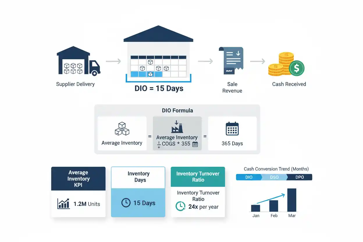
Days inventory outstanding, commonly abbreviated DIO, estimates the average number of days inventory remains on hand before being sold or otherwise moving through the cost-of-sales cycle represented by the calculation.
A common days inventory outstanding formula is:
Days Inventory Outstanding = Average Inventory ÷ Cost of Goods Sold × Number of Days
If a business maintains $500,000 of average inventory while annual cost of goods sold is $3,650,000:
DIO = $500,000 ÷ $3,650,000 × 365
DIO = 50 days
The business therefore carries approximately 50 days of inventory under the assumptions used.
DIO is useful because inventory can absorb substantial amounts of working capital. However, a lower number is not automatically better. Inventory must be sufficient to meet customer demand, production requirements, seasonal peaks, supplier lead times, and operational risk.
For that reason, days inventory outstanding works best alongside inventory turnover, the cash conversion cycle, working capital, and the broader business finance framework.
What Is Days Inventory Outstanding?
Days inventory outstanding estimates how many days of inventory a company carries relative to the cost of inventory moving through its operations.
The metric is sometimes called inventory days, days inventory held, or days sales of inventory, depending on the analytical convention.
Its purpose is straightforward:
How long, on average, does inventory remain tied up before it moves into cost of goods sold?
If DIO equals 30 days, the company carries roughly one month of inventory relative to the cost flow represented by the calculation.
If DIO equals 120 days, the inventory balance represents roughly four months of cost of goods sold.
That does not automatically mean the company literally stores every item for exactly 30 or 120 days. DIO is based on aggregate accounting balances and provides an average operating indicator rather than item-level shelf age.
Days Inventory Outstanding Formula
The common annual formula is:
DIO = Average Inventory ÷ Cost of Goods Sold × 365
For a quarterly calculation, the analyst can use the appropriate number of days in the period when the numerator and denominator cover the same period.
A generalized formula is:
DIO = Average Inventory ÷ Cost of Goods Sold for the Period × Days in the Period
Average inventory is often calculated using beginning and ending inventory:
Average Inventory = (Beginning Inventory + Ending Inventory) ÷ 2
Suppose beginning inventory is $700,000 and ending inventory is $900,000.
Average Inventory = ($700,000 + $900,000) ÷ 2
Average Inventory = $800,000
If annual cost of goods sold is $4 million:
DIO = $800,000 ÷ $4,000,000 × 365
DIO = 73 days
The company carries approximately 73 days of inventory under the calculation.
Why Use Average Inventory?
Cost of goods sold represents activity across an accounting period.
Ending inventory represents a balance at one specific date.
Using average inventory helps align the stock measure with the period-based cost flow.
Suppose a retailer begins the year with $400,000 of inventory and finishes with $1 million after building stock for a large seasonal event.
Using only the $1 million year-end balance could materially overstate the inventory level that existed during much of the year.
A simple average would be:
Average Inventory = ($400,000 + $1,000,000) ÷ 2
Average Inventory = $700,000
For highly seasonal or volatile businesses, monthly or quarterly average inventory can provide a better denominator than averaging only the first and last day of the year.
Days Inventory Outstanding Example
Assume a distributor reports:
Beginning inventory = $900,000
Ending inventory = $1,100,000
Annual cost of goods sold = $5,000,000
Calculate average inventory:
Average Inventory = ($900,000 + $1,100,000) ÷ 2
Average Inventory = $1,000,000
Now calculate DIO:
DIO = $1,000,000 ÷ $5,000,000 × 365
DIO = 73 days
The distributor carries approximately 73 days of inventory.
If the business can safely reduce that number while maintaining product availability and sales, less capital may need to remain tied up in inventory.
If lower DIO results from product shortages, however, the apparent efficiency improvement can harm revenue.
What Does a High DIO Mean?
A relatively high days inventory outstanding means the company’s inventory balance is large compared with the cost of goods sold moving through the period.
Several explanations are possible.
The business may deliberately maintain substantial safety stock. Supplier lead times may be long. Production may require extended processing. Management may be preparing for a seasonal peak or expected shortage.
A high DIO can also indicate slower demand, excessive purchasing, obsolete stock, forecasting errors, or products that no longer sell efficiently.
The number identifies the relationship. It does not identify the cause.
Management should therefore examine inventory composition, product-level aging, sales patterns, purchasing commitments, and write-down risk before concluding that a high DIO represents inefficiency.
What Does a Low DIO Mean?
A low DIO generally means the company holds less inventory relative to its cost of goods sold.
That can reflect fast-selling products, efficient supply chains, short supplier lead times, strong demand forecasting, or lean inventory management.
It can reduce the amount of working capital tied up in stock.
Yet extremely low inventory days can create a different problem.
If the company does not carry enough products or materials, it may experience stockouts, missed sales, delayed production, emergency shipping costs, or greater vulnerability to supplier disruption.
Inventory efficiency should therefore balance capital use with service and operational resilience.
What Is a Good Days Inventory Outstanding?
There is no universal good DIO.
A grocery retailer handling perishable goods should have very different inventory economics from an industrial-equipment distributor whose products can remain in stock for months.
A manufacturer may need raw materials, work in process, and finished goods simultaneously.
A made-to-order service may carry virtually no traditional inventory.
The strongest benchmark usually combines the company’s historical DIO with comparable businesses that have similar product, supply-chain, seasonality, and inventory characteristics.
A raw cross-industry comparison has little analytical value.
Days Inventory Outstanding vs Inventory Turnover
DIO and inventory turnover describe closely related inventory efficiency from opposite directions.
Inventory turnover commonly uses:
Inventory Turnover = Cost of Goods Sold ÷ Average Inventory
DIO commonly uses:
DIO = Average Inventory ÷ Cost of Goods Sold × 365
If inventory turnover is calculated consistently for a full year, the two measures are approximately reciprocal:
DIO ≈ 365 ÷ Inventory Turnover
Suppose inventory turnover is 5 times per year.
DIO ≈ 365 ÷ 5
DIO ≈ 73 days
Higher inventory turnover normally corresponds with lower DIO.
Lower turnover normally corresponds with higher DIO.
A 2026 SEC filing from MSC Industrial Direct states that its inventory turnover metric is calculated using cost of goods sold divided by inventory based on a trailing average, illustrating the real-world use of average inventory in turnover analysis.
Inventory Turnover Example Converted to DIO
Suppose annual cost of goods sold is $6 million and average inventory is $1.2 million.
Inventory turnover:
Inventory Turnover = $6,000,000 ÷ $1,200,000
Inventory Turnover = 5 times
Convert to approximate days:
DIO = 365 ÷ 5
DIO = 73 days
The business turns its average inventory approximately five times annually and carries roughly 73 days of inventory.
Both metrics express the same broad operating relationship in different units.
Managers may find days easier to connect with lead times and planning, while turnover can be easier for comparison across financial statements.
DIO and Cost of Goods Sold
Cost of goods sold belongs in the denominator because DIO is intended to compare inventory with the cost flow associated with selling that inventory.
The IRS illustrates the relationship between beginning inventory, purchases, goods available for sale, ending inventory, and cost of goods sold in its current small-business tax guidance.
A simplified inventory-cost relationship is:
Beginning Inventory + Net Inventory Purchases and Relevant Costs − Ending Inventory = Cost of Goods Sold
The exact accounting treatment depends on the business and applicable accounting requirements.
For DIO analysis, the key point is that inventory is compared with the related cost flow, not sales revenue.
Using revenue instead of cost of goods sold would mix an asset measured at cost with a sales measure that contains margin.
DIO and Gross Profit
Gross profit connects revenue with cost of goods sold:
Gross Profit = Revenue − Cost of Goods Sold
DIO focuses on the inventory side of that relationship.
A company can increase gross profit while DIO deteriorates if inventory accumulates faster than sales.
For example, strong margins do not make excess stock disappear.
Conversely, a business can have highly efficient inventory movement while operating on narrow margins.
Inventory efficiency and profitability therefore need to be analyzed separately before being connected.
DIO and Gross Margin
Gross margin measures gross profit relative to revenue.
DIO measures inventory relative to cost of goods sold.
Suppose two retailers both have 60-day DIO.
One earns a 50% gross margin, while the other earns 15%.
Their inventory timing is similar, but the economics of each sale differ substantially.
Likewise, two businesses can have identical margins but very different inventory requirements.
Neither metric substitutes for the other.
DIO and the Cash Conversion Cycle
Days inventory outstanding forms the first component of the cash conversion cycle.
Cash Conversion Cycle = DIO + Days Sales Outstanding − Days Payable Outstanding
Suppose:
DIO = 70 days
DSO = 35 days
DPO = 45 days
Cash Conversion Cycle = 70 + 35 − 45
Cash Conversion Cycle = 60 days
If DIO falls from 70 to 55 days while the other measures remain unchanged:
New Cash Conversion Cycle = 55 + 35 − 45
New Cash Conversion Cycle = 45 days
The 15-day inventory improvement reduces the modeled cash conversion cycle by 15 days.
This is why DIO is more than a warehouse metric. It can directly affect the amount of time operating cash remains tied up.
DIO and Days Sales Outstanding
Days sales outstanding begins where inventory economics can end for a credit sale.
DIO measures the inventory-holding phase.
DSO measures the customer-collection phase.
Suppose goods remain in inventory for 50 days and the customer then takes 40 days to pay.
Before supplier-payment effects:
Inventory and Receivable Period = 50 + 40
Inventory and Receivable Period = 90 days
Inventory efficiency can therefore improve without solving a slow-receivables problem.
A company needs to understand both stages.
DIO and Days Payable Outstanding
Days payable outstanding measures supplier-payment timing.
Supplier credit can offset part of the cash tied up in inventory.
Suppose the company carries 80 days of inventory but pays suppliers in 60 days.
Ignoring the receivable period, the company must finance roughly 20 days between those two components under the simplified relationship.
If suppliers shorten terms to 30 days, the financing requirement increases.
Purchasing inventory is therefore not only a merchandising or production decision. Payment terms also influence its cash impact.
DIO and Working Capital
Inventory is commonly a major component of working capital for product-based companies.
A simple working-capital formula is:
Working Capital = Current Assets − Current Liabilities
When inventory rises, current assets can rise.
That may improve the absolute working-capital balance while simultaneously tying more cash into stock.
This creates an important distinction:
More working capital is not automatically more liquid working capital.
A warehouse full of slow-moving goods is less immediately usable than an equivalent amount of cash.
DIO and the Current Ratio
Inventory is ordinarily included among current assets when classified as current, so higher inventory can increase the current ratio.
Suppose:
Cash and receivables = $400,000
Inventory = $600,000
Other current assets = $100,000
Current liabilities = $550,000
Current assets equal $1.1 million.
Current Ratio = $1,100,000 ÷ $550,000
Current Ratio = 2.0
If another $200,000 of inventory accumulates while liabilities remain unchanged:
New Current Ratio = $1,300,000 ÷ $550,000
New Current Ratio ≈ 2.36
The ratio improved mathematically.
If the additional inventory accumulated because demand collapsed, actual operating quality may have worsened.
DIO can help expose that problem.
DIO and the Quick Ratio
The quick ratio generally excludes inventory.
That makes it useful when the current ratio is heavily influenced by inventory balances.
Suppose a company has a current ratio of 2.5 but a quick ratio of only 0.8.
A large portion of current-asset coverage is therefore dependent on inventory and other assets excluded from the quick calculation.
If DIO is also rising sharply, management has another reason to examine whether inventory is genuinely liquid.
DIO and the Cash Ratio
The cash ratio narrows liquidity even further by focusing on cash and cash equivalents relative to current liabilities.
Inventory does not directly improve the cash ratio.
A company can therefore report a strong current ratio because of large inventory while simultaneously maintaining a weak cash ratio.
DIO helps explain how quickly some of that inventory may move toward becoming cash.
Still, selling inventory can create accounts receivable rather than immediate cash, so DIO should not be interpreted as a direct cash-conversion promise.
DIO and Cash Flow Forecasting
Cash flow forecasting turns planned inventory purchases into actual expected cash dates.
DIO provides a high-level efficiency indicator.
Suppose annual DIO is 60 days.
That does not tell management exactly when a $500,000 supplier invoice must be paid next month.
The forecast provides that detail.
Conversely, a cash forecast may show a large inventory purchase but not make it immediately obvious whether overall inventory efficiency is deteriorating.
The two tools complement one another.
DIO and Free Cash Flow
Inventory growth can consume cash and affect free cash flow.
Suppose inventory rises by $1 million because the company builds stock ahead of expansion.
Cash can decline even though the inventory remains an asset on the balance sheet.
If that stock later sells efficiently, the cash investment may be productive.
If it becomes obsolete, the company may lose both liquidity and economic value.
DIO can therefore help explain why increasing profits do not always produce equivalent cash generation.
DIO and Burn Rate
Inventory-heavy startups and growth businesses can experience higher burn rate when they must purchase stock before receiving customer cash.
Suppose an e-commerce business aggressively expands its product selection.
Inventory purchases rise by $300,000 per month while customer sales ramp more slowly.
Net cash burn can increase even if management expects the inventory to produce profitable future sales.
Tracking DIO helps distinguish between a planned temporary inventory build and an increasingly inefficient stock position.
DIO and Cash Runway
Large inventory requirements can shorten cash runway.
Suppose a company has $2 million of available cash and otherwise burns $100,000 per month.
A $600,000 inventory build reduces immediately available cash before the related products are sold.
If the runway model ignores that purchase timing, it can materially overstate the number of months available.
Businesses with large or seasonal stock requirements should therefore model inventory cash flows explicitly rather than relying on a constant average burn rate.
How Inventory Growth Can Hide Behind Revenue Growth
A fast-growing business may report impressive revenue while inventory grows even faster.
Suppose revenue rises 20%, but average inventory rises 60%.
If cost of goods sold grows more slowly than inventory, DIO can increase substantially.
That means more capital is being committed for each unit of product moving through the company.
The increase might be intentional—for example, to support a new location or product range—but management should understand the reason.
Revenue growth alone does not prove inventory efficiency.
DIO and Asset Turnover
Inventory is part of total assets, so excessive inventory can also influence asset turnover.
Asset turnover measures revenue relative to average total assets.
If inventory rises substantially without proportional sales growth, the total asset base increases and asset turnover can weaken.
DIO provides a more focused diagnosis by isolating the inventory component.
A company with declining asset turnover may therefore examine inventory days, receivables, fixed assets, and other balance-sheet accounts to find the source.
DIO and Contribution Margin
Contribution margin tells management how much each sale contributes after relevant variable costs.
A high contribution margin can justify carrying some slower-moving inventory when the eventual economics are strong.
However, a high-margin product that almost never sells can still represent poor use of working capital.
Management needs both dimensions:
How much does the product contribute when it sells?
and
How long does cash remain tied up before that sale occurs?
DIO addresses the second question.
DIO and Break-Even Analysis
Inventory is not itself part of the standard break-even analysis formula.
However, inventory decisions affect the cash needed to support the sales volume required for break-even.
Suppose a company needs to sell 10,000 units each month to cover fixed costs.
If it must carry four months of inventory to guarantee availability, it may need to finance approximately 40,000 units of stock across the relevant operating process.
A mathematically attractive break-even level can therefore require substantial working capital.
Seasonal Inventory and DIO
Seasonality can distort DIO substantially.
A toy retailer, clothing company, agricultural supplier, or holiday-goods distributor may intentionally accumulate stock ahead of peak demand.
Inventory can rise sharply before revenue arrives.
If DIO is measured at the peak inventory date, it may look unusually high.
After the selling season, the same company can report much lower inventory days.
For seasonal businesses, comparing equivalent periods and using more frequent average inventory balances is particularly important.
DIO for Manufacturers
Manufacturers can hold several inventory categories simultaneously: raw materials, work in process, and finished goods.
Total DIO combines those balances into one high-level measure.
If total DIO rises, management should determine which category caused the increase.
Raw materials may have accumulated because of supplier-risk planning.
Work in process may indicate production bottlenecks.
Finished goods may be increasing because customer demand weakened.
A single total DIO cannot distinguish these causes.
DIO for Retailers
Retail inventory tends to consist mainly of goods held for sale.
The relevant risks can include overstocks, seasonal leftovers, changing fashion or technology, shrinkage, markdowns, and product obsolescence.
A rising DIO can therefore have pricing consequences.
Products may ultimately require discounts to move.
That can reduce gross margin even if the inventory was originally expected to sell at full price.
Inventory days and margin trends should therefore be reviewed together.
DIO for Perishable Inventory
Perishable goods require particularly careful inventory-day interpretation.
A food retailer, pharmaceutical distributor, or other business handling products with limited usable lives can face direct economic losses when inventory remains too long.
The relevant DIO target may therefore be much shorter than for durable industrial goods.
Aggregate DIO can also hide aging risk if fast-moving products offset extremely slow-moving items.
Item-level and category-level inventory aging remains necessary.
Obsolete Inventory and DIO
Inventory can remain on the balance sheet even when its economic prospects have weakened, subject to applicable accounting measurement and impairment requirements.
SEC-filed companies disclose inventory impairments when inventory values must be reduced, demonstrating that recorded inventory is not automatically worth its original carrying amount indefinitely.
A rising DIO can serve as one warning sign, particularly when accompanied by slowing sales or increasing markdowns.
However, DIO by itself cannot determine whether inventory is obsolete.
That requires product-level operational and accounting analysis.
Inventory Accounting Methods and DIO
Inventory accounting methods can affect reported inventory balances and cost of goods sold.
For example, companies may use methods such as FIFO, LIFO where permitted and applicable, or average-cost approaches depending on their circumstances and accounting framework.
A 2026 SEC filing documents a company changing its U.S. product inventory costing method from average cost to LIFO, illustrating that inventory accounting choices can change reported values used in financial analysis.
This matters when comparing DIO between companies.
Two businesses with similar physical inventory flows can report somewhat different accounting relationships if their costing methods differ materially.
DIO comparisons should therefore be interpreted with financial-statement policies in mind.
DIO and Inventory Valuation
DIO measures the relationship between reported average inventory and cost of goods sold.
It does not independently determine whether inventory is correctly valued.
Inventory can be affected by purchase costs, manufacturing costs, write-downs, vendor allowances, discounts, and applicable valuation methods.
IRS guidance describes purchased merchandise inventory at cost as including invoice price adjusted for trade discounts plus certain associated costs, reinforcing that inventory carrying amounts represent accounting cost rather than retail selling price.
This is another reason revenue should not replace cost of goods sold in the standard DIO formula.
How to Reduce Days Inventory Outstanding
DIO can decline when average inventory falls relative to cost of goods sold.
Operationally, that can result from better demand forecasting, tighter purchasing, shorter supplier lead times, smaller order quantities, improved production scheduling, stronger product assortment decisions, faster fulfillment, or removal of obsolete stock.
However, inventory should not be reduced blindly.
Suppose cutting stock lowers DIO from 60 days to 25 days but produces frequent product shortages.
The ratio improved, but revenue and customer service may suffer.
The goal is economically efficient inventory, not the smallest possible DIO.
Improving DIO Through Demand Forecasting
Better forecasting can reduce unnecessary stock while preserving availability.
Suppose a company routinely purchases 10,000 units because historical forecasts overestimate demand.
Actual demand averages only 7,000.
Reducing purchasing toward realistic demand can lower average inventory without affecting sales.
The resulting improvement can release working capital and potentially reduce storage or obsolescence costs.
Forecast accuracy should therefore be connected with inventory decisions rather than used only as a sales-planning metric.
Improving DIO Through Supplier Lead Times
Long supplier lead times often force companies to carry more safety stock.
If lead times can be shortened reliably, the company may need less inventory to protect against supply interruption.
However, choosing the fastest supplier is not always optimal.
Prices, quality, reliability, payment terms, geography, minimum order quantities, and supply-chain risk also matter.
DIO provides the financial effect of inventory holdings, while procurement decisions determine whether reducing those holdings is operationally sensible.
Improving DIO Through Product Rationalization
Some businesses accumulate inventory because they carry too many slow-selling products.
SKU-level analysis can identify products that consume inventory investment while generating little contribution.
Removing or reducing those items can improve DIO and release cash.
Yet product rationalization must consider strategic assortment.
Some slow-moving products support customer relationships or complementary purchases.
Again, inventory efficiency needs economic context.
Can DIO Be Zero?
A conventional DIO can approach zero when a business carries very little inventory relative to cost of goods sold.
Some businesses may operate with minimal physical inventory because products move immediately, suppliers ship directly to customers, or the business is primarily service-based.
For a company with no relevant inventory, DIO may not be a meaningful operating metric at all.
Trying to benchmark an inventory-free software company against a physical retailer would serve little purpose.
Can DIO Be Negative?
Under the conventional formula, DIO normally should not be negative because both inventory and cost of goods sold are ordinarily nonnegative values.
A negative result generally indicates unusual data, adjustments, a denominator problem, or an inappropriate application of the formula.
The inputs should be reviewed rather than treating a negative DIO as a normal inventory-efficiency result.
How Much Cash Can Lower DIO Release?
A rough estimate can be developed by connecting inventory days with daily cost of goods sold.
Suppose annual COGS is $7.3 million.
Average daily COGS is:
Daily COGS = $7,300,000 ÷ 365
Daily COGS = $20,000
If DIO falls sustainably by 10 days:
Approximate Inventory Reduction = $20,000 × 10
Approximate Inventory Reduction = $200,000
Under stable cost flow, the company may require approximately $200,000 less average inventory.
That does not mean a $200,000 cash inflow automatically appears immediately. Purchasing commitments, payment timing, inventory mix, taxes, and other operational factors affect how and when cash is released.
DIO Trend Analysis
A single DIO figure provides limited context.
Suppose a company reports:
Year 1: 48 days
Year 2: 55 days
Year 3: 72 days
The rising trend deserves investigation.
Potential explanations include slower sales, deliberate inventory investment, supply-chain protection, a new product launch, weaker forecasting, purchasing errors, or obsolete stock.
Now consider:
Year 1: 75 days
Year 2: 60 days
Year 3: 45 days
The declining trend suggests faster inventory movement.
Management should still verify that service levels and sales were preserved.
Trend direction is informative; operational cause determines whether the change is favorable.
Common Days Inventory Outstanding Mistakes
One mistake is using ending inventory when the balance fluctuated substantially during the period.
Another is dividing inventory by revenue rather than the related cost-of-sales measure.
Businesses may also compare annual DIO with quarterly competitor figures without adjusting for the number of days.
Seasonal balances can distort comparisons.
Accounting methods can affect the reported inventory and COGS values.
Perhaps the biggest interpretation mistake is assuming lower DIO is always better.
Excess inventory consumes capital, but insufficient inventory can cost the company sales.
Limitations of Days Inventory Outstanding
DIO compresses an entire inventory system into one average.
It does not identify obsolete products.
It does not reveal stockouts.
It does not show supplier reliability.
It cannot distinguish raw materials from finished goods unless those components are analyzed separately.
It may also be affected by accounting policies and seasonality.
A company with thousands of products can have a reasonable overall DIO while a small group of products creates substantial aging risk.
The metric should therefore be used as a diagnostic indicator, not a replacement for detailed inventory management.
How to Analyze DIO Properly
Begin with the formula using a consistent period and a representative average inventory balance.
Compare the result with the company’s historical trend.
Then compare it with genuinely similar businesses where definitions are reasonably comparable.
Break the inventory balance into relevant categories.
Review turnover, aging, sales trends, purchasing patterns, stockouts and write-downs.
Next, connect DIO with DSO and DPO through the cash conversion cycle.
Finally, examine what inventory levels mean for cash flow and working capital.
A useful DIO analysis explains both how quickly inventory is moving and whether that speed makes economic sense for the business.
Frequently Asked Questions
What is days inventory outstanding?
Days inventory outstanding estimates the average number of days inventory remains on hand relative to the cost of goods sold during the analyzed period.
What does DIO stand for?
DIO stands for days inventory outstanding.
What is the days inventory outstanding formula?
DIO = Average Inventory ÷ Cost of Goods Sold × Number of Days
How do you calculate average inventory?
A simple calculation is:
Average Inventory = (Beginning Inventory + Ending Inventory) ÷ 2
More frequent average balances can be useful when inventory is volatile or seasonal.
What does a DIO of 60 mean?
It means the business carries approximately 60 days of inventory relative to its cost of goods sold under the calculation.
Is a lower DIO better?
Usually, lower DIO indicates faster inventory movement and less capital tied up in stock, but excessively low inventory can cause stockouts or production problems.
What is a good DIO?
There is no universal target. Appropriate inventory days depend on industry, product life, supplier lead times, seasonality, customer demand, production requirements, and business strategy.
What is the difference between DIO and inventory turnover?
Inventory turnover shows how many times average inventory moves through cost of goods sold during a period. DIO expresses approximately the same relationship as a number of days.
How are DIO and inventory turnover related?
For a consistent annual calculation:
DIO ≈ 365 ÷ Inventory Turnover
Does high DIO mean inventory is obsolete?
Not automatically. High DIO can result from seasonality, safety stock, long production cycles, supply-chain planning, slow demand, or obsolete products. Inventory aging must be examined separately.
Is DIO part of the cash conversion cycle?
Yes.
Cash Conversion Cycle = DIO + DSO − DPO
Can a company reduce DIO too much?
Yes. Excessively lean inventory can lead to shortages, lost sales, production interruptions, emergency purchasing, and lower customer service levels.
Final Perspective
Days inventory outstanding converts an inventory balance into a more intuitive operating measure:
DIO = Average Inventory ÷ Cost of Goods Sold × Days in the Period
If the result is 60 days, the company carries approximately 60 days of inventory relative to the cost flow represented by the calculation.
But the financial objective is not to drive that number toward zero.
Inventory exists for a reason. It supports sales, production continuity, customer availability and resilience against supply uncertainty.
Too much inventory ties up cash and can increase storage, markdown and obsolescence risk.
Too little inventory can stop the company from selling.
The useful question is therefore not:
“How low can we make DIO?”
It is:
“Are we holding the right amount of inventory for the demand, lead times and operating risks we face—and how much cash does that inventory strategy require?”
That is where days inventory outstanding becomes a meaningful business-finance metric rather than another isolated ratio.