The degree of combined leverage, or DCL, measures how sensitive a company’s earnings available to shareholders are to a percentage change in sales when both operating leverage and financial leverage are considered.
In its most direct form:
Degree of Combined Leverage = % Change in EPS ÷ % Change in Sales
DCL can also be expressed as the product of operating and financial leverage:
DCL = Degree of Operating Leverage × Degree of Financial Leverage
Suppose a company has a degree of operating leverage of 2.5 and a degree of financial leverage of 1.4.
DCL = 2.5 × 1.4
DCL = 3.5
At that operating point, a 1% change in sales is associated with an approximately 3.5% change in earnings per share under the assumptions of the leverage model.
Therefore, if sales increase by 10%:
Estimated EPS Change = 10% × 3.5
Estimated EPS Change = 35%
The relationship works in both directions. A 10% sales decline can produce an approximately 35% decline in EPS under the same simplified assumptions.
That amplification is the central purpose of the degree of combined leverage. It captures the effect of fixed operating costs and fixed financing costs within one sensitivity measure.
Operating leverage measures how strongly operating income responds to sales changes, and higher fixed operating costs can increase that sensitivity. Financial leverage adds the effect of debt and other fixed financing obligations on shareholder earnings.
Within business finance, DCL is therefore best understood as an earnings-sensitivity measure rather than simply another debt ratio.
What Is Degree of Combined Leverage?
Degree of combined leverage measures the combined amplification created by a company’s operating cost structure and financing structure.
Sales change first.
Because some operating expenses are fixed, operating income can change by a greater percentage than sales.
Then financial obligations such as interest expense can cause earnings available to shareholders to change by an even greater percentage than operating income.
The sequence is:
Sales → EBIT → Earnings to Equity
Operating leverage governs the first amplification.
Financial leverage governs the second.
Combined leverage captures both.
This distinction matters because two companies generating the same revenue can have very different earnings sensitivity depending on fixed costs and debt.
Degree of Combined Leverage Formula
The broad sensitivity formula is:
DCL = Percentage Change in EPS ÷ Percentage Change in Sales
If sales increase 8% and EPS increases 24%:
DCL = 24% ÷ 8%
DCL = 3.0
The company’s EPS changed approximately three times as much as sales over the measured relationship.
A second formula is:
DCL = DOL × DFL
where:
DOL = Degree of Operating Leverage
DFL = Degree of Financial Leverage
Suppose:
DOL = 2.0
DFL = 1.5
DCL = 2.0 × 1.5
DCL = 3.0
Both approaches describe the same combined sensitivity when the underlying definitions and assumptions are consistent.
Contribution-Based DCL Formula
For a simplified single-period cost-volume-profit model, combined leverage can also be expressed using contribution margin.
A useful form is:
DCL = Total Contribution Margin ÷ Earnings Before Tax
When preferred dividends, taxes, unusual financing structures, or alternative EPS definitions are involved, the formula can require adjustment.
For a simplified company:
Sales = $1,000,000
Variable costs = $600,000
Fixed operating costs = $250,000
Interest expense = $50,000
Contribution margin is:
Contribution Margin = $1,000,000 − $600,000
Contribution Margin = $400,000
EBIT is:
EBIT = $400,000 − $250,000
EBIT = $150,000
Earnings before tax are:
EBT = $150,000 − $50,000
EBT = $100,000
Combined leverage becomes:
DCL = $400,000 ÷ $100,000
DCL = 4.0
Under this simplified model, a 1% sales movement produces an approximately 4% movement in pre-tax earnings attributable through the leverage chain.
Complete Degree of Combined Leverage Example
Consider a business with:
Sales = $2,000,000
Variable costs = $1,200,000
Fixed operating costs = $500,000
Interest expense = $100,000
First calculate contribution margin:
Contribution Margin = Sales − Variable Costs
Contribution Margin = $2,000,000 − $1,200,000
Contribution Margin = $800,000
Next calculate EBIT:
EBIT = Contribution Margin − Fixed Operating Costs
EBIT = $800,000 − $500,000
EBIT = $300,000
Then calculate earnings before tax:
EBT = EBIT − Interest
EBT = $300,000 − $100,000
EBT = $200,000
Degree of operating leverage is:
DOL = Contribution Margin ÷ EBIT
DOL = $800,000 ÷ $300,000
DOL ≈ 2.67
Degree of financial leverage is:
DFL = EBIT ÷ EBT
DFL = $300,000 ÷ $200,000
DFL = 1.50
Therefore:
DCL = 2.67 × 1.50
DCL ≈ 4.00
The same result appears directly:
DCL = Contribution Margin ÷ EBT
DCL = $800,000 ÷ $200,000
DCL = 4.00
The company’s earnings sensitivity is therefore approximately four times its sales sensitivity at this operating point.
What Does a DCL of 4 Mean?
A DCL of 4 means a 1% change in sales is associated with an approximately 4% change in the relevant shareholder-earnings measure under the model.
If sales rise 5%:
Expected Earnings Change ≈ 5% × 4
Expected Earnings Change ≈ 20%
If sales fall 5%:
Expected Earnings Change ≈ −5% × 4
Expected Earnings Change ≈ −20%
This is why high combined leverage can be attractive during expansion and dangerous during contraction.
The leverage itself does not determine whether sales rise or fall.
It determines how strongly earnings respond once sales move.
Degree of Combined Leverage and Sales Growth
Combined leverage can make modest revenue growth produce much larger earnings growth.
Suppose DCL is 3.2.
Sales rise by 10%.
Expected Earnings Change ≈ 10% × 3.2
Expected Earnings Change ≈ 32%
That amplification can create strong shareholder earnings growth once the company has enough sales to cover its fixed operating and financial commitments.
Actual results can differ if prices, product mix, variable-cost rates, fixed costs, interest expense, taxes, or other assumptions change.
DCL is therefore a local sensitivity measure rather than a universal forecast multiplier.
DCL and Falling Sales
The same leverage works against the business when sales decline.
Suppose:
DCL = 5
Sales decline = 8%
Estimated Earnings Change = −8% × 5
Estimated Earnings Change = −40%
A relatively modest revenue decline can therefore produce a much larger earnings decline.
This asymmetric business concern—not mathematical asymmetry—is why leverage risk becomes particularly important near break-even levels.
When earnings are already small, fixed operating and financing commitments consume a large portion of the remaining contribution.
Degree of Operating Leverage
The first component of DCL is degree of operating leverage, or DOL.
A common formula is:
DOL = Contribution Margin ÷ EBIT
Another interpretation is:
DOL = % Change in EBIT ÷ % Change in Sales
OpenStax defines operating leverage as the sensitivity of net operating income to percentage changes in sales and explains that higher fixed-cost structures generally create greater operating leverage.
Suppose contribution margin is $600,000 and EBIT is $300,000.
DOL = $600,000 ÷ $300,000
DOL = 2.0
A 1% sales change is therefore associated with approximately a 2% EBIT change under the modeled relationship.
Degree of Financial Leverage
The second component is degree of financial leverage, or DFL.
In a simplified financing structure:
DFL = EBIT ÷ (EBIT − Interest Expense)
Since:
EBT = EBIT − Interest Expense
the formula becomes:
DFL = EBIT ÷ EBT
Suppose:
EBIT = $300,000
Interest expense = $100,000
DFL = $300,000 ÷ ($300,000 − $100,000)
DFL = $300,000 ÷ $200,000
DFL = 1.50
Financial leverage reflects how fixed financing costs can amplify changes in operating earnings for equity holders. Debt financing creates contractual claims that must generally be satisfied before residual earnings accrue to equity.
Why DCL Equals DOL × DFL
The relationship follows the earnings chain.
Operating leverage measures:
% Change in EBIT ÷ % Change in Sales
Financial leverage measures:
% Change in EPS ÷ % Change in EBIT
Multiply them:
(% Change in EBIT ÷ % Change in Sales) × (% Change in EPS ÷ % Change in EBIT)
The percentage change in EBIT cancels:
DCL = % Change in EPS ÷ % Change in Sales
Therefore:
DCL = DOL × DFL
This makes combined leverage an intuitive bridge between the company’s operating cost structure and financing structure.
Operating Leverage vs Financial Leverage vs Combined Leverage
The three concepts answer different questions.
Operating leverage asks:
How sensitive is operating profit to changes in sales?
Financial leverage asks:
How sensitive are shareholder earnings to changes in operating profit?
Combined leverage asks:
How sensitive are shareholder earnings to changes in sales after both effects are included?
Suppose:
DOL = 2
DFL = 1.5
Then:
DCL = 3
Sales changing 10% implies approximately:
EBIT Change ≈ 10% × 2 = 20%
and:
EPS Change ≈ 20% × 1.5 = 30%
Combined directly:
EPS Change ≈ 10% × 3 = 30%
DCL and Fixed Costs
Fixed costs are a primary source of operating leverage.
Imagine two businesses with identical revenue.
Company A outsources most operations and pays costs that vary with sales.
Company B owns facilities, employs substantial permanent staff and carries high fixed infrastructure expense.
When sales rise, Company B may not need to increase those fixed expenses proportionately.
A larger share of additional contribution can therefore reach EBIT.
When sales fall, the same fixed costs remain.
That creates greater earnings sensitivity.
Public companies frequently describe improving operating leverage as revenue grows across relatively fixed infrastructure or operating expense bases.
DCL and Variable Costs
Variable costs reduce contribution margin as sales occur.
A business with high variable costs and low fixed costs tends to have lower operating leverage than an otherwise similar company with low variable costs and high fixed costs.
Suppose two businesses each generate $1 million in sales.
Company A:
Variable cost = $800,000
Fixed cost = $100,000
Contribution:
$1,000,000 − $800,000 = $200,000
EBIT:
$200,000 − $100,000 = $100,000
DOL:
$200,000 ÷ $100,000 = 2.0
Company B:
Variable cost = $500,000
Fixed cost = $400,000
Contribution:
$500,000
EBIT:
$100,000
DOL:
$500,000 ÷ $100,000 = 5.0
Both produce the same EBIT, but Company B has much greater operating leverage.
DCL and Contribution Margin
Contribution margin is central to the simplified DCL formula because it measures the amount available after variable costs to cover fixed operating costs and financing effects.
Suppose selling price rises while variable cost remains unchanged.
Contribution margin increases.
If fixed costs and debt remain unchanged, operating earnings can become less vulnerable once the company moves farther above break-even.
Conversely, falling contribution margins can push the company closer to its fixed-cost threshold and increase leverage sensitivity.
Contribution margin therefore provides the economic bridge between sales and EBIT.
DCL and Break-Even Point
Break-even point matters because operating leverage generally becomes particularly high when EBIT is small near the operating break-even threshold.
Consider:
Contribution margin = $520,000
Fixed operating costs = $500,000
EBIT = $20,000
DOL:
DOL = $520,000 ÷ $20,000
DOL = 26
The company is only slightly above operating break-even.
A relatively small sales movement can therefore produce a very large percentage change in EBIT.
Once sales increase and EBIT becomes substantially larger, DOL typically falls under the same cost structure.
DCL Changes With Sales Volume
Degree of combined leverage is not necessarily a permanent characteristic of a company.
Suppose contribution margin is $600,000, fixed operating costs are $400,000 and interest is $50,000.
EBIT:
$600,000 − $400,000 = $200,000
EBT:
$200,000 − $50,000 = $150,000
DCL:
$600,000 ÷ $150,000 = 4.0
Now sales increase enough for contribution margin to reach $900,000 while fixed operating costs and interest remain unchanged.
New EBIT:
$900,000 − $400,000 = $500,000
New EBT:
$500,000 − $50,000 = $450,000
New DCL:
$900,000 ÷ $450,000 = 2.0
The business still has fixed costs and debt, but its earnings are less sensitive at the higher operating level.
DCL Near Financial Break-Even
Financial leverage becomes extreme when EBIT approaches interest expense.
Suppose:
EBIT = $110,000
Interest = $100,000
EBT = $10,000
DFL:
DFL = $110,000 ÷ $10,000
DFL = 11
The company has little earnings cushion above its financing cost.
Small changes in EBIT can create very large percentage changes in earnings before tax.
If operating leverage is also high, combined leverage can become extremely large.
This is one reason debt can materially increase shareholder earnings volatility. Debt ratios and other solvency measures are important partly because borrowing introduces fixed repayment and interest obligations.
DCL When Earnings Before Tax Are Zero
Suppose EBIT equals interest expense.
EBT equals zero.
The simplified formula becomes:
DCL = Contribution Margin ÷ 0
Division by zero is undefined.
This is economically meaningful.
At the financial break-even point, infinitesimal changes around zero earnings can create extremely large percentage changes.
The percentage-sensitivity interpretation therefore becomes unstable.
DCL should not be treated mechanically when the denominator is zero or extremely close to zero.
Can DCL Be Negative?
Yes, depending on the company’s earnings position and formula used.
Suppose the company has positive contribution but negative earnings before tax.
Contribution margin = $500,000
EBT = −$100,000
DCL = $500,000 ÷ −$100,000
DCL = −5
However, negative DCL is not interpreted in the same intuitive way as a normal positive leverage ratio.
The company is operating in a loss region where percentage changes around negative earnings can behave differently from conventional profitable-company sensitivity.
The underlying income statement should be analyzed directly.
Is a Higher Degree of Combined Leverage Better?
Not automatically.
Higher DCL creates greater upside sensitivity when sales increase.
It also creates greater downside sensitivity when sales fall.
Suppose Company A has DCL of 2.
Company B has DCL of 6.
A 10% sales increase implies approximately:
Company A:
10% × 2 = 20% earnings increase
Company B:
10% × 6 = 60% earnings increase
But a 10% sales decline implies:
Company A:
−20%
Company B:
−60%
Company B has greater earnings potential from sales expansion but also greater earnings risk.
What Is a Good Degree of Combined Leverage?
There is no universal ideal DCL.
Appropriate combined leverage depends on revenue stability, industry cyclicality, margins, fixed operating expenses, borrowing costs, customer concentration and management’s risk tolerance.
A business with stable recurring revenue can potentially support more leverage than a highly cyclical company.
Likewise, a fast-growing company with substantial fixed infrastructure may intentionally accept high operating leverage in expectation of scaling revenue.
DCL should therefore be compared with the company’s own operating conditions rather than an arbitrary benchmark.
DCL and Debt Ratio
The debt ratio measures debt relative to total assets.
DCL measures earnings sensitivity.
They can move differently.
Suppose two companies each have a 50% debt ratio.
One has stable fixed-rate financing at low interest expense.
The other pays much higher interest.
Their balance-sheet leverage appears similar, but DFL—and therefore DCL—can differ substantially.
Debt ratio measures how much leverage exists on the balance sheet.
DCL measures how leverage affects earnings sensitivity.
DCL and Debt-to-Equity Ratio
The debt-to-equity ratio compares debt with shareholder equity.
A higher D/E ratio can indicate greater financial leverage, but it does not determine DFL directly.
Interest expense depends on borrowing rates, maturity structure and debt instruments.
Two companies with identical D/E ratios can therefore have different DCL values.
Balance-sheet leverage and income-statement sensitivity need separate measurement.
DCL and Interest Coverage
Interest coverage provides a particularly useful complement to DCL.
A common formula is:
Interest Coverage = EBIT ÷ Interest Expense
Suppose:
EBIT = $500,000
Interest = $100,000
Interest Coverage = 5×
Financial leverage is relatively moderate under the simplified model:
DFL = $500,000 ÷ $400,000
DFL = 1.25
Now suppose EBIT falls to $150,000 while interest remains $100,000.
Interest Coverage = 1.5×
DFL becomes:
DFL = $150,000 ÷ $50,000
DFL = 3.0
As the earnings cushion above interest shrinks, financial leverage sensitivity increases sharply.
DCL and EBIT
EBIT sits directly between operating and financial leverage.
Sales and operating costs determine EBIT.
Interest expense then affects earnings below EBIT.
That makes EBIT the dividing line in the combined-leverage chain:
Sales → Operating Leverage → EBIT → Financial Leverage → EPS
A company can therefore reduce combined leverage either by altering its operating cost structure or its financing structure.
The next article in the master sequence is the dedicated EBIT page, so EBIT calculation itself remains there rather than being duplicated here.
DCL and EBITDA
EBITDA can help describe operating performance before depreciation and amortization, interest and taxes.
However, DCL commonly uses EBIT within its financial-leverage component because interest follows EBIT in the simplified income-statement sequence.
A company with substantial depreciation can have EBITDA far above EBIT.
Using EBITDA mechanically in place of EBIT would therefore change the leverage calculation.
The master plan assigns EBITDA its own dedicated page immediately after EBIT, preserving that distinction.
DCL and Operating Margin
Operating margin measures operating income relative to sales.
A company with thin operating margins can experience substantial earnings sensitivity because a relatively small sales decline may eliminate much of its EBIT.
Suppose revenue is $10 million and operating margin is only 3%.
EBIT is:
EBIT = $10,000,000 × 3%
EBIT = $300,000
If the business also has substantial fixed costs and debt, combined leverage can be high.
A strong revenue base does not by itself guarantee low earnings sensitivity.
DCL and Gross Margin
Gross margin can influence contribution economics, but it is not identical to contribution margin.
Gross margin is based on revenue and cost of goods sold.
Contribution margin separates variable costs from sales.
A business can have strong gross margin but still carry substantial variable selling costs.
DCL analysis requires costs to be classified according to how they behave within the leverage model, not simply where they appear in external financial statements.
DCL and Operating Leverage in Real Businesses
Operating leverage is not merely theoretical. Public companies routinely describe situations where growing revenue over relatively fixed infrastructure or operating expenses improves profitability. For example, recent SEC-filed disclosures discuss leveraging fixed corporate, technology, or operating cost bases as revenue scales.
The exact degree of leverage still depends on actual cost behavior.
A cost labeled fixed today can become variable at a larger scale if new facilities, staff or systems become necessary.
DCL therefore works within a relevant operating range rather than across unlimited sales growth.
Relevant Range and DCL
Cost-volume-profit relationships assume a range within which underlying cost behavior remains reasonably valid.
OpenStax defines the relevant range as the activity range within which current productive capacity and cost assumptions apply.
Suppose a factory can produce up to 100,000 units without additional facilities.
Within that range, rent and major equipment costs may remain fixed.
At 101,000 units, management might need a second facility.
Fixed costs then step upward.
A DCL calculated below that threshold should not be extrapolated blindly beyond it.
DCL and Pricing
Pricing changes can alter contribution margin and therefore operating leverage.
Suppose a company sells 20,000 units at $100 with variable cost of $60.
Contribution per unit is:
$100 − $60 = $40
Total contribution:
20,000 × $40 = $800,000
If price increases to $110 and volume remains unchanged:
New Contribution per Unit = $110 − $60 = $50
Total Contribution = $1,000,000
If fixed operating and financing costs remain unchanged, EBIT and EBT increase, potentially moving the company farther from break-even and reducing DCL at the new operating level.
However, a price change can also affect sales volume.
The leverage model cannot predict customer demand.
DCL and Discounts
Discounts can reduce contribution margin and move a company closer to its operating break-even point.
Suppose price falls from $100 to $90 while variable cost remains $60.
Contribution per unit falls from $40 to $30.
If fixed costs remain unchanged, more sales are required to produce the same EBIT.
Operating leverage can therefore increase if the discount compresses the operating earnings cushion.
A promotion that increases revenue can still increase risk when unit contribution deteriorates too far.
DCL and Sales Mix
Companies selling multiple products can have different contribution margins across products.
A shift toward low-contribution products can reduce aggregate contribution even when total revenue remains unchanged.
That can raise operating leverage if EBIT falls closer to fixed costs.
Conversely, a shift toward high-contribution products can increase EBIT and reduce leverage sensitivity at the new operating point.
Sales mix therefore matters when applying DCL to multi-product businesses.
DCL and Capacity Expansion
A company may deliberately increase fixed costs to create additional capacity.
Suppose management leases a second facility.
Fixed operating costs rise immediately.
Revenue may take time to fill the new capacity.
During that period, operating leverage and DCL can increase.
If sales eventually scale successfully across the larger capacity base, the company can benefit from stronger earnings growth.
Capacity investments therefore often create a period where leverage risk rises before the expected operating benefit appears.
DCL and Automation
Automation can change cost structure by replacing some variable labor or processing costs with fixed technology or equipment costs.
Suppose variable cost per unit falls while depreciation, software commitments or fixed infrastructure costs rise.
At high sales volume, the automated model can produce stronger operating profits.
At low sales volume, the larger fixed-cost base can create greater downside sensitivity.
Automation decisions therefore can change DOL and, consequently, DCL.
DCL and Outsourcing
Outsourcing can have the opposite effect.
A company may replace fixed internal capacity with per-unit supplier charges.
Variable costs rise, while fixed operating costs decline.
This can reduce operating leverage.
The company sacrifices some upside margin at high volume in exchange for greater flexibility when sales fall.
Combined leverage provides one framework for understanding that risk-return trade-off.
DCL and Business Cyclicality
Cyclical companies can face particular risk from high combined leverage.
When economic conditions weaken, sales can decline sharply.
If operating fixed costs remain and debt interest continues, shareholder earnings can contract much faster than revenue.
A company in a stable essential-service market may tolerate a similar DCL more comfortably because its revenue varies less.
The acceptable amount of leverage therefore depends partly on the volatility of the underlying sales base.
DCL and Customer Concentration
Customer concentration can amplify the practical risk associated with DCL.
Suppose one customer generates 30% of revenue.
If that customer leaves, the business experiences a large sales decline immediately.
High combined leverage can transform that revenue loss into an even larger earnings decline.
A company with diversified revenue can face less probability of such a sudden sales shock even with the same mathematical DCL.
DCL and Cash Flow
DCL is primarily an earnings-sensitivity concept.
It does not measure cash flow directly.
Depreciation, working capital, capital expenditure, taxes and financing principal payments can cause cash movements to differ from accounting earnings.
A company can therefore show improving EPS while still experiencing weak cash generation.
Operating cash flow and free cash flow should be analyzed separately.
DCL and Cash Flow Forecasting
Cash flow forecasting can help management determine whether a highly leveraged earnings structure also creates liquidity risk.
Suppose DCL indicates substantial downside sensitivity.
A downside revenue scenario can then be translated into projected EBIT, interest obligations and cash balances.
This connection converts an abstract leverage ratio into a practical stress test.
DCL identifies sensitivity.
The cash forecast identifies whether the resulting financial position can be funded.
DCL and Burn Rate
For a company already consuming cash, high operating leverage can make burn rate deteriorate quickly when sales weaken.
Fixed payroll, facilities or infrastructure continue consuming cash while customer receipts decline.
Debt interest can add another fixed cash requirement.
A revenue shock can therefore increase both accounting losses and cash consumption.
DCL does not calculate burn, but it can identify a structure where earnings are particularly sensitive to the same sales shock.
DCL and Cash Runway
Cash runway becomes especially important for highly leveraged growth companies.
Suppose a downside scenario reduces sales 15%.
If DCL is 4:
Estimated Earnings Change ≈ −15% × 4
≈ −60%
The resulting cash impact depends on working capital, noncash costs and financing payments, but the earnings sensitivity provides an early warning.
Management can then model how the downside case changes runway.
DCL and Business Valuation
Business valuation depends partly on expected cash flows and risk.
High leverage can magnify earnings growth during favorable periods, but it can also make forecasts more volatile and shareholder outcomes riskier.
A buyer or investor should therefore distinguish between growth produced by expanding underlying economics and growth amplified primarily by leverage.
DCL is not a valuation formula.
It helps explain the risk profile behind projected earnings.
DCL and Return on Equity
Return on equity can rise when financial leverage amplifies shareholder earnings.
Suppose operating profits rise while debt financing keeps the equity base relatively small.
ROE can expand rapidly.
However, high DCL means the same structure can push ROE downward quickly if sales weaken.
High ROE generated through leverage should therefore be distinguished from high ROE generated through strong operating economics alone.
DCL and Economic Value Added
Economic value added examines whether operating profit after tax exceeds the cost of capital employed.
Combined leverage asks a different question.
A highly leveraged strategy can increase EPS sensitivity without necessarily creating additional economic value.
If borrowed capital is invested in low-return projects, leverage can amplify shareholder risk without generating returns above the capital cost.
The next several articles in the Business Finance sequence deepen these related earnings, capital and leverage concepts.
Can a Company Reduce DCL?
Yes.
A company can reduce operating leverage by lowering fixed operating costs relative to variable costs.
It can reduce financial leverage by lowering debt or other fixed financing commitments.
Increasing operating earnings while fixed costs and interest remain constant can also reduce DCL at the new operating level.
For example, higher contribution margin can move the company farther above break-even.
Debt repayment can reduce interest expense.
The appropriate strategy depends on why leverage is high.
Should a Company Always Reduce Combined Leverage?
No.
Leverage can be deliberately accepted because it creates stronger upside economics.
A factory with substantial fixed capacity can earn excellent incremental margins after break-even.
Borrowing can finance productive investment without requiring additional equity.
The trade-off is risk.
Reducing every fixed commitment can sacrifice scale economics and potential shareholder return.
Combined leverage should therefore be managed rather than automatically minimized.
Degree of Combined Leverage Trend Analysis
Suppose DCL changes:
Year 1: 2.2
Year 2: 3.1
Year 3: 5.0
The rising trend means shareholder earnings have become increasingly sensitive to sales movements under the model.
Possible causes include higher fixed operating costs, more debt, higher interest expense, declining contribution margins or weaker EBIT.
A falling DCL can reflect stronger operating earnings, lower fixed costs, debt repayment, lower interest or improved contribution.
The headline direction should always be traced to its operating and financial components.
Common Degree of Combined Leverage Mistakes
A common mistake is assuming DCL is constant across every sales level.
It is not.
Another is confusing combined leverage with the debt-to-equity ratio.
D/E measures capital structure, while DCL measures earnings sensitivity.
Using EBITDA instead of EBIT without adjusting the model can also produce inconsistent financial-leverage calculations.
The measure becomes unstable near zero earnings.
Finally, DCL should not be interpreted as a guaranteed prediction that EPS will move by exactly the calculated multiple.
It assumes relevant cost, price and financing relationships remain sufficiently stable around the modeled operating point.
Limitations of Degree of Combined Leverage
DCL simplifies complex business economics.
It assumes meaningful relationships among sales, variable costs, fixed operating costs and financing costs.
Actual cost behavior can change with volume.
Prices and sales mix can shift.
Interest rates can change.
Tax effects can complicate EPS.
New equity issuance can change shares outstanding.
Large investments can change fixed costs.
Consequently, DCL is most useful as a sensitivity measure within a defined operating range, not as an unlimited forecasting multiplier.
How to Analyze DCL Properly
Start with the income statement and classify costs according to the model.
Calculate contribution margin.
Determine EBIT.
Identify relevant fixed financing costs.
Calculate DOL and DFL independently.
Then multiply them to confirm DCL.
Test the direct contribution-to-earnings formula where appropriate.
Next, model both revenue growth and revenue contraction.
Compare the result with debt ratios, interest coverage and cash-flow scenarios.
Finally, determine whether the company’s sales stability is consistent with the amount of earnings sensitivity it carries.
The objective is not to find the lowest or highest DCL.
It is to understand whether the company’s operating and financing structure creates an acceptable balance between earnings growth potential and downside risk.
Frequently Asked Questions
What is degree of combined leverage?
Degree of combined leverage measures how sensitive shareholder earnings are to a percentage change in sales after both operating leverage and financial leverage are considered.
What does DCL stand for?
DCL stands for degree of combined leverage.
What is the degree of combined leverage formula?
The broad sensitivity formula is:
DCL = % Change in EPS ÷ % Change in Sales
It can also be calculated as:
DCL = DOL × DFL
How do you calculate DCL from contribution margin?
In a simplified structure:
DCL = Contribution Margin ÷ Earnings Before Tax
The exact formulation may require adjustments for more complex financing or EPS structures.
What does a DCL of 3 mean?
A DCL of 3 means a 1% change in sales is associated with an approximately 3% change in the relevant shareholder-earnings measure under the modeled assumptions.
Is higher DCL better?
Not automatically. Higher DCL increases upside earnings sensitivity when sales grow and downside earnings sensitivity when sales fall.
What is a good degree of combined leverage?
There is no universal ideal. Appropriate DCL depends on sales stability, industry cyclicality, margins, fixed costs, debt and financing capacity.
What is the difference between DOL and DCL?
DOL measures EBIT sensitivity to sales. DCL measures shareholder-earnings sensitivity to sales after both operating and financial leverage.
What is the difference between DFL and DCL?
DFL measures shareholder-earnings sensitivity to EBIT. DCL combines that financial effect with operating leverage starting from sales.
What is the difference between DCL and debt-to-equity ratio?
Debt-to-equity compares debt with shareholder equity. DCL measures how operating and financial fixed costs amplify changes in shareholder earnings when sales move.
Can degree of combined leverage be negative?
Yes, mathematically, when the relevant earnings denominator is negative. However, negative DCL requires careful interpretation because the company is operating in a loss region.
Why does DCL become very high near break-even?
Because EBIT or earnings before tax becomes small relative to contribution margin. A small absolute change can therefore create a very large percentage change in earnings.
Final Perspective
The degree of combined leverage connects the entire earnings chain:
Sales → EBIT → Shareholder Earnings
Operating leverage amplifies the first step.
Financial leverage amplifies the second.
Together:
DCL = DOL × DFL
or:
DCL = % Change in EPS ÷ % Change in Sales
A DCL of 4 means that a 1% movement in sales is associated with an approximately 4% movement in shareholder earnings under the assumptions of the model.
That amplification can be powerful when revenue grows.
It can be equally severe when revenue falls.
The useful question is therefore not:
“Is high combined leverage good or bad?”
It is:
“How stable are our sales, how much fixed operating cost do we carry, how much fixed financing cost do we carry, and can the business absorb the downside if revenue moves against us?”
That is the real purpose of the degree of combined leverage: measuring how operating structure and financing structure combine to magnify the financial consequences of changes in sales.