Volume variance measures the financial effect of actual activity being different from the activity level used in a budget, standard, or planning model.
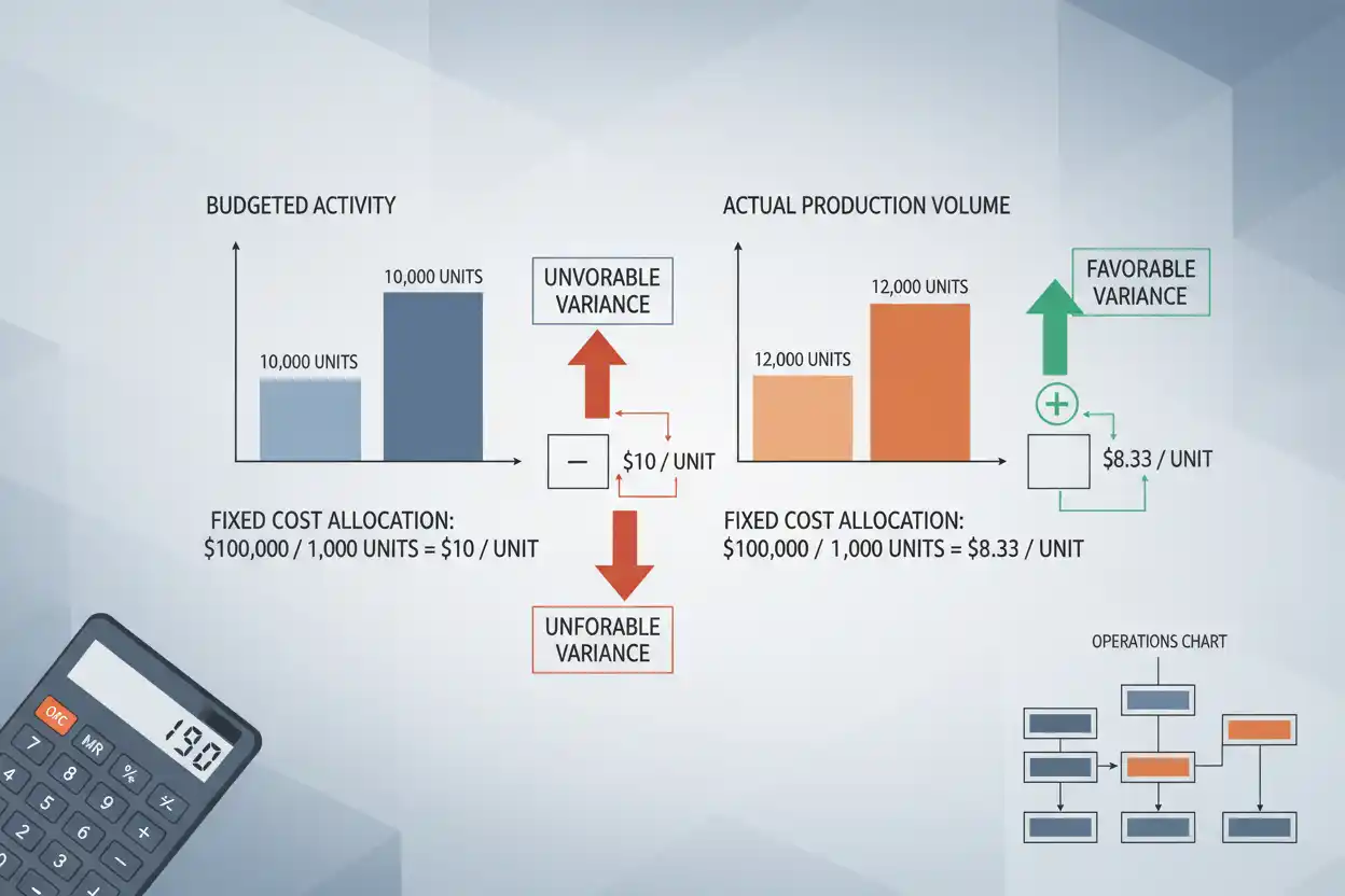
If a manufacturer expected to produce 10,000 units but actually produced 12,000, the difference is 2,000 units. When each unit carries a standard contribution, fixed-overhead allocation, or other relevant benchmark amount, that volume difference can be translated into a dollar variance.
A general form is:
Volume Variance = (Actual Volume − Budgeted Volume) × Standard Amount per Unit
Suppose actual production is 12,000 units, budgeted production is 10,000 units, and the relevant standard amount is $8 per unit:
Volume Variance = (12,000 − 10,000) × $8 = $16,000
The interpretation of that $16,000 depends on what the $8 benchmark represents. Volume variance is therefore not one universal accounting formula with one universal favorable/unfavorable meaning. The underlying cost, revenue, contribution, or overhead framework must be identified first.
What Is Volume Variance?
Volume variance isolates the effect of how much activity occurred compared with how much activity was expected.
Businesses forecast activity in many forms:
production units, sales units, labor hours, machine hours, customer transactions, occupied rooms, deliveries, subscriptions, or another measurable activity base.
If the actual level differs from the plan, some financial results can differ even when unit prices and unit costs remain unchanged.
Suppose a factory expects to produce 50,000 units but actually produces only 40,000.
The 10,000-unit shortfall can affect fixed-cost absorption, production efficiency analysis, inventory levels, sales availability, and other measures.
Volume variance attempts to isolate the effect of that activity difference rather than combining it with price or unit-cost changes.
Volume Variance Formula
A broad analytical formula is:
Volume Variance = (Actual Activity − Budgeted Activity) × Standard Financial Amount per Activity Unit
Where:
Actual activity is the number of units, hours, transactions, or other activity actually achieved.
Budgeted activity is the planned or standard activity level.
Standard amount per unit is the financial value assigned to each activity unit for the specific variance being measured.
For a simple unit-volume analysis:
Unit Volume Difference = Actual Units − Budgeted Units
If actual units equal 9,000 and budgeted units equal 10,000:
Unit Volume Difference = 9,000 − 10,000 = −1,000 Units
If the relevant standard amount is $6 per unit:
Volume Variance = −1,000 × $6 = −$6,000
Whether that result is labeled favorable or unfavorable depends on the economic context.
Volume Variance Example
Suppose a business budgets production of 20,000 units.
Actual production reaches 23,000 units.
The standard amount used for the analysis is $5 per unit.
Volume difference:
23,000 − 20,000 = 3,000 Units
Dollar variance:
3,000 × $5 = $15,000
The company has a $15,000 volume effect relative to the budget under this model.
If the $5 represents expected contribution from each additional unit and all incremental units can be sold profitably, the higher volume could be favorable.
If the $5 represents fixed overhead being allocated differently, interpretation requires the specific overhead-variance framework.
The arithmetic alone does not determine the business meaning.
Volume Variance in Units
Sometimes the most useful measure is simply the difference in physical activity:
Volume Variance in Units = Actual Volume − Budgeted Volume
Suppose:
Budgeted Sales = 50,000 Units
Actual Sales = 46,000 Units
Then:
Volume Variance = 46,000 − 50,000 = −4,000 Units
Actual volume is 4,000 units below plan.
Percentage difference:
−4,000 ÷ 50,000 × 100 = −8%
Actual unit volume is 8% below budget.
This physical measure can be useful before assigning any financial value to the difference.
Positive and Negative Volume Variance
A positive volume difference means actual activity exceeded the benchmark:
Actual Volume > Budgeted Volume
A negative difference means actual activity was lower:
Actual Volume < Budgeted Volume
The favorable or unfavorable label depends on the metric.
Higher sales volume may usually be favorable if unit economics remain positive.
Higher production volume can be unfavorable if the business produces inventory that cannot be sold.
Lower production can be rational if demand is weaker than expected and management avoids unnecessary stock.
A sign should therefore not be interpreted independently of the underlying activity.
Sales Volume Example
Suppose a retailer expected to sell 30,000 units at a standard contribution amount of $12 per unit.
Actual sales volume is 27,000 units.
Difference:
27,000 − 30,000 = −3,000 Units
Volume effect:
−3,000 × $12 = −$36,000
The business generated $36,000 less contribution than expected from the unit-volume difference under the assumptions.
This isolates volume.
If the selling price or variable cost also changed, those changes should be analyzed separately rather than folded into the same volume variance.
Production Volume Example
Suppose a manufacturer planned production of 100,000 units but completed 90,000.
The fixed production cost budget is $500,000, implying a simplified planned fixed-cost amount of:
$500,000 ÷ 100,000 = $5 per Planned Unit
Production falls short by:
90,000 − 100,000 = −10,000 Units
Using $5 as the relevant standard amount:
−10,000 × $5 = −$50,000
The lower production volume means the planned activity base was not achieved.
Within an overhead-absorption framework, lower-than-planned production can leave fixed production costs spread over fewer units.
Volume Variance and Unit Cost
Unit cost often changes when production volume differs from plan because fixed costs are distributed across a different number of units.
Suppose fixed manufacturing cost is $400,000.
At a planned volume of 100,000 units:
Fixed Cost per Unit = $400,000 ÷ 100,000 = $4
Actual production is only 80,000 units:
Actual Average Fixed Cost per Unit = $400,000 ÷ 80,000 = $5
The same fixed cost is now spread across fewer units.
Average fixed cost per unit rises by:
$5 − $4 = $1 per Unit
This does not mean unit cost and volume variance are the same metric. The unit-cost page owns the per-unit calculation; volume variance isolates the effect of activity differing from the benchmark.
Volume Variance and Fixed Costs
Volume matters most when costs do not change proportionally with activity.
Suppose a factory has $600,000 of annual fixed cost.
Budgeted production:
120,000 Units
Budgeted fixed cost per unit:
$600,000 ÷ 120,000 = $5
Actual production:
150,000 Units
Average fixed cost per actual unit:
$600,000 ÷ 150,000 = $4
Higher volume spreads the same fixed cost over 30,000 more units.
That can improve average unit economics, assuming the additional production is useful and saleable.
Producing more simply to spread fixed cost is not automatically economically sound because excess inventory can create carrying costs and obsolescence.
Volume Variance and Variable Costs
Variable costs behave differently.
Suppose material cost is $3 per unit.
At 10,000 units:
Total Variable Cost = $30,000
At 12,000 units:
Total Variable Cost = $36,000
Total cost increases because volume increases, but cost per unit remains $3 if price and usage efficiency are unchanged.
The $6,000 increase in total variable cost is not necessarily a cost-control problem. It can simply reflect 2,000 additional units of activity.
Variance analysis is useful because it separates more activity from more cost per unit.
Volume Variance vs. Price Variance
Price variance isolates the difference between actual and standard unit prices.
Volume variance isolates the difference in activity quantity.
Suppose a business budgets:
10,000 Units × $20 = $200,000
Actual results are:
12,000 Units × $22 = $264,000
Total difference:
$264,000 − $200,000 = $64,000
Part of that difference comes from selling or purchasing more units.
Part comes from the $2 unit-price difference.
Combining the two into one unexplained $64,000 variance hides the underlying drivers.
Good variance analysis separates price and volume effects rather than treating all movement as one category.
Volume Variance vs. Cost Variance
Cost variance is broader.
A total cost difference can be created by:
- different activity volume;
- different unit prices;
- different material usage;
- labor efficiency;
- product mix;
- overhead differences; or
- several factors at once.
Volume variance isolates one of those drivers.
Suppose actual total cost is $110,000 and budgeted cost is $100,000.
A $10,000 unfavorable total cost variance does not prove costs were poorly controlled.
If actual output was 20% above budget, the business might actually have spent less per unit even though total cost increased.
Example: Higher Cost but Favorable Volume Economics
Suppose:
Budget
10,000 Units
Total Cost = $100,000
Budget cost per unit:
$10
Actual
12,000 Units
Total Cost = $114,000
Actual cost per unit:
$114,000 ÷ 12,000 = $9.50
Total cost is $14,000 above budget.
Yet unit cost is $0.50 lower.
The higher total expenditure is largely associated with greater output.
Looking only at total cost would make performance appear worse than the per-unit economics suggest.
Example: Lower Cost but Unfavorable Volume Economics
The opposite can occur.
Budget:
10,000 Units
Total Cost = $100,000
Actual:
7,000 Units
Total Cost = $85,000
Total spending is $15,000 below budget.
But:
Actual Cost per Unit = $85,000 ÷ 7,000 ≈ $12.14
Average unit cost is much higher than the planned $10.
Lower total spending does not necessarily indicate better efficiency when activity falls substantially.
Volume Variance and Labor Productivity
Revenue per employee and other productivity metrics can help explain why activity volume changed.
Suppose a factory expects 5 units of output per labor hour and uses 10,000 labor hours.
Expected production:
5 × 10,000 = 50,000 Units
Actual labor productivity improves to 5.5 units per hour with the same labor input:
Actual Output = 5.5 × 10,000 = 55,000 Units
Production is 5,000 units above the original expectation.
The volume increase may therefore originate from productivity improvement rather than additional labor hours.
Volume variance identifies the activity difference; productivity analysis explains one possible cause.
Volume Variance and Revenue per Employee
Suppose a company budgets $10 million of revenue with 100 employees:
Budget Revenue per Employee = $100,000
Actual revenue reaches $11 million with the same average workforce:
Actual Revenue per Employee = $110,000
Revenue volume or pricing effects have increased sales relative to headcount.
The revenue per employee metric provides a workforce-normalized perspective, while volume variance isolates activity relative to the plan.
Revenue can rise because of price even when physical volume is flat, so these metrics should not be treated as interchangeable.
Volume Variance and Sales per Square Foot
A retailer can also experience changes in sales per square foot because sales volume differs from plan.
Suppose a 10,000-square-foot store budgets $3 million in annual sales:
Budget Sales per Square Foot = $300
Actual sales are only $2.7 million:
Actual Sales per Square Foot = $270
If selling prices are unchanged, lower unit volume may explain much of the $30-per-square-foot decline.
If prices changed, the relationship becomes more complex.
Volume variance isolates quantity; sales per square foot measures revenue productivity of physical retail space.
Volume Variance and Safety Stock
Safety stock can influence whether unexpected sales volume is actually fulfilled.
Suppose demand is 20% higher than forecast.
If sufficient inventory is available, actual sales volume can exceed plan.
If stock runs out, customer demand may exist without becoming actual sales volume.
A sales-volume variance can therefore partly reflect inventory availability rather than customer interest alone.
This distinction matters when management investigates why volume was below forecast.
Volume Variance and Reorder Point
A poorly calibrated reorder point can also reduce achieved volume.
Suppose expected demand is strong, but the business repeatedly orders inventory too late.
Stockouts can prevent the company from fulfilling demand.
The resulting sales-volume shortfall may look like a demand problem even though the actual cause is replenishment timing.
Variance investigation should therefore distinguish market volume from fulfilled volume.
Volume Variance and Inventory Buildup
Higher production volume is not always favorable.
Suppose a factory budgets production of 100,000 units and sales of 100,000 units.
Actual production is 120,000 units, but sales remain 100,000.
The additional 20,000 units increase inventory rather than customer sales.
If unit production cost is $15:
Additional Inventory Production = 20,000 × $15 = $300,000
The company has committed another $300,000 of product cost to stock.
A favorable production-volume variance can therefore coexist with poor working-capital economics.
Volume Variance and Inventory Carrying Cost
Higher-than-required production can raise inventory carrying cost.
Suppose the additional $300,000 of inventory remains on hand and the annual carrying-cost rate is 20%.
Estimated annual carrying burden:
$300,000 × 20% = $60,000
The production-volume increase might improve fixed-cost absorption while creating $60,000 of estimated annual carrying cost.
This is why maximizing production volume is not the same as maximizing economic value.
Volume Variance and Trial Balance
The trial balance contains the accounting balances that ultimately support financial reporting.
Volume variance, however, also requires operational or budget data.
The actual cost may come from accounting records, while:
- standard quantities;
- planned production;
- expected sales units; and
- budgeted activity
come from management planning systems.
A balanced trial balance does not prove that production volume matched budget.
The two serve different purposes: bookkeeping control versus management analysis.
Production Volume and Capacity
Suppose normal facility capacity is 100,000 units.
Management budgets 90,000 but actual demand requires 105,000.
The 15,000-unit favorable difference versus budget may push production beyond normal capacity.
That can trigger:
- overtime;
- temporary labor;
- expedited materials;
- maintenance pressure;
- quality issues; or
- outsourced production.
The financial value per additional unit may therefore change as the business moves into a different operating range.
A constant standard amount can become less realistic near capacity limits.
Volume Variance and Operating Income
Higher volume can improve operating income when additional sales generate sufficient gross profit without an equivalent increase in operating expenses.
Suppose 5,000 additional units are sold.
Contribution before fixed operating costs is $10 per unit:
Additional Contribution = 5,000 × $10 = $50,000
If additional operating expenses are only $15,000:
Incremental Operating Income = $50,000 − $15,000 = $35,000
Higher volume improves operating income by $35,000 in this simplified example.
The volume variance itself should still remain distinct from the full operating-income calculation.
Volume Variance and Revenue
Revenue is influenced by both price and quantity.
A simple formula is:
Revenue = Price × Volume
Suppose budget revenue assumes:
10,000 Units × $50 = $500,000
Actual volume is 12,000 units and selling price remains $50:
Actual Revenue = $600,000
The $100,000 revenue increase comes entirely from volume:
2,000 Additional Units × $50 = $100,000
If actual selling price also changes, the revenue variance should be decomposed rather than assigned entirely to volume.
Volume Variance Percentage
A simple percentage measure is:
Volume Variance % = (Actual Volume − Budgeted Volume) ÷ Budgeted Volume × 100
Suppose:
Budgeted Volume = 80,000 Units
Actual Volume = 92,000 Units
Then:
Volume Variance % = (92,000 − 80,000) ÷ 80,000 × 100
Volume Variance % = 15%
Actual activity was 15% above plan.
If actual volume is 68,000 instead:
(68,000 − 80,000) ÷ 80,000 × 100 = −15%
Actual activity was 15% below plan.
Multi-Period Volume Variance Example
Suppose:
| Month | Budget Units | Actual Units | Unit Difference |
|---|---|---|---|
| January | 10,000 | 9,500 | -500 |
| February | 10,500 | 10,800 | +300 |
| March | 11,000 | 12,000 | +1,000 |
| April | 11,500 | 12,600 | +1,100 |
Total budget volume:
43,000 Units
Total actual volume:
44,900 Units
Cumulative difference:
44,900 − 43,000 = 1,900 Units
Cumulative percentage variance:
1,900 ÷ 43,000 × 100 ≈ 4.42%
Actual volume is approximately 4.42% above the four-month plan.
Looking across several periods can reveal whether a single-month variance is temporary or part of a sustained trend.
Investigating an Unfavorable Volume Variance
When activity is below plan, management should identify the cause before deciding what to change.
For sales volume, possible explanations include weak demand, stockouts, competitor activity, pricing changes, sales execution, product quality, seasonality, or an unrealistic forecast.
For production volume, causes can include equipment downtime, labor shortages, material shortages, quality failures, poor scheduling, lower demand, or deliberate output reductions.
The correct response differs completely depending on the cause.
Increasing production would not solve a demand problem.
Increasing marketing would not solve a machine-capacity problem.
Investigating a Favorable Volume Variance
Higher-than-budgeted activity also deserves investigation.
Strong sales volume may indicate better demand, successful marketing, improved distribution, higher retention, or stronger sales execution.
Higher production can result from improved labor productivity, reduced downtime, better scheduling, or deliberate inventory buildup.
Management should determine whether the higher activity is profitable and sustainable.
A favorable label should never end the analysis.
Common Volume Variance Mistakes
One common mistake is treating any increase in total cost as unfavorable without adjusting for higher activity.
Another is mixing price changes with volume changes.
Businesses can also use an incorrect standard amount per unit, making the dollar variance economically meaningless.
Another error is automatically labeling higher production as favorable even when the extra units accumulate in inventory.
Management may also compare volume periods with different seasonality or capacity conditions.
Finally, the actual and budget quantities must use the same units and cover the same period.
Frequently Asked Questions
What is volume variance in simple terms?
Volume variance measures the effect of actual activity being different from the amount of activity expected in a budget or standard.
What is the volume variance formula?
A broad formula is:
Volume Variance = (Actual Volume − Budgeted Volume) × Standard Amount per Unit
The precise financial interpretation depends on the type of variance being measured.
How do you calculate volume variance in units?
Use:
Actual Units − Budgeted Units
If actual volume is 12,000 and budgeted volume is 10,000:
Unit Volume Variance = 2,000 Units
How do you calculate volume variance percentage?
Volume Variance % = (Actual Volume − Budgeted Volume) ÷ Budgeted Volume × 100
Is positive volume variance always favorable?
No.
Higher sales volume may be favorable, but higher production that simply creates excess inventory can be economically unfavorable.
Is negative volume variance always unfavorable?
No.
Lower output can be rational when demand is weaker than planned and producing additional inventory would create unnecessary cost.
Is volume variance the same as price variance?
No.
Price variance isolates differences in unit price.
Volume variance isolates differences in activity quantity.
Is volume variance the same as cost variance?
No.
Cost variance is broader and can contain price, volume, usage, efficiency, mix, and other effects.
Why does production volume affect unit cost?
Fixed costs are distributed across the units produced. When production falls, the same fixed cost can be spread over fewer units, increasing average fixed cost per unit.
Can higher total costs occur with better unit economics?
Yes.
If output rises faster than total cost, total spending can increase while cost per unit falls.
Can lower total cost indicate worse performance?
Yes.
If activity drops significantly, total cost can fall while cost per unit rises and revenue opportunities are lost.
How can inventory affect sales volume variance?
Stockouts can prevent customer demand from becoming completed sales, producing an unfavorable sales-volume result even when underlying demand is strong.
Why should volume variance be investigated with operational data?
Accounting figures show the financial effect, but operational data explains whether the cause was demand, capacity, productivity, inventory, supplier performance, or another factor.
What is the main purpose of volume variance?
Its main purpose is to separate the financial impact of activity level from changes caused by price, unit cost, efficiency, or other variables.