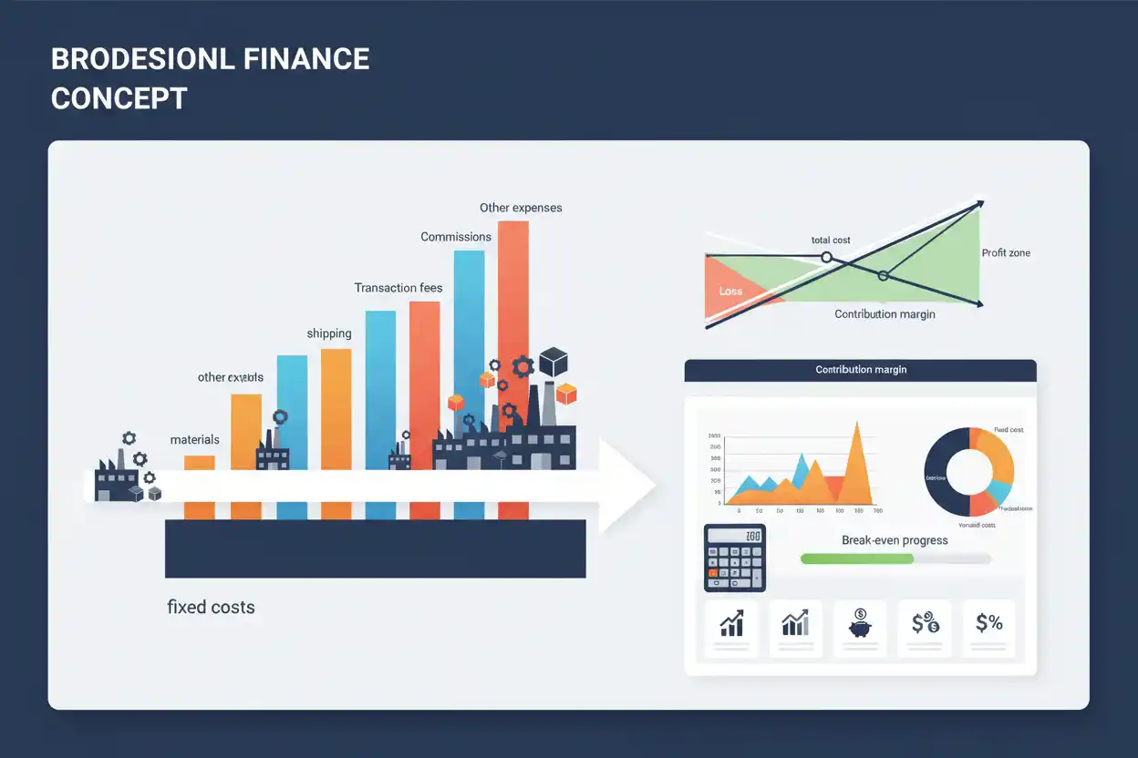
Variable costs are expenses that change as business activity changes. When a company produces or sells more units, total variable costs generally rise. When activity falls, total variable costs generally decline.
The basic formula is:
Total Variable Cost = Variable Cost per Unit × Number of Units
Suppose a manufacturer incurs $12 of variable cost for every product it makes and produces 10,000 units.
Total Variable Cost = $12 × 10,000
Total Variable Cost = $120,000
If production increases to 15,000 units while the variable cost remains $12 per unit:
Total Variable Cost = $12 × 15,000
Total Variable Cost = $180,000
Total variable cost increased by $60,000 because the company produced 5,000 additional units.
Understanding variable costs is central to business finance because they affect contribution margin, break-even volume, pricing, profitability, unit economics, cash requirements, and decisions about whether additional sales create economic value.
What Are Variable Costs?
Variable costs are costs that change with a relevant level of business activity.
Depending on the company, the activity driver might be:
units produced;
products sold;
customer orders;
transactions processed;
miles driven;
labor hours;
deliveries completed;
or another measurable activity.
For example, a retailer may pay a payment-processing fee every time a customer purchases an item. More transactions generate more processing fees.
A manufacturer may consume additional raw materials every time another unit is produced.
A delivery company may incur additional courier compensation and fuel-related expense as delivery volume increases.
The defining feature is the relationship between cost and activity.
Variable Cost Formula
For a simple unit-based model:
Total Variable Cost = Variable Cost per Unit × Activity Volume
If total variable cost and production volume are known:
Variable Cost per Unit = Total Variable Cost ÷ Number of Units
Suppose a business incurs $240,000 of variable costs while producing 20,000 units.
Variable Cost per Unit = $240,000 ÷ 20,000
Variable Cost per Unit = $12
If the $12 unit cost remains stable and production rises to 25,000 units:
Expected Variable Cost = $12 × 25,000
Expected Variable Cost = $300,000
The formula is straightforward when cost changes proportionately with activity.
Real businesses can be more complicated because unit costs can change as volume, supplier pricing, labor efficiency, or capacity conditions change.
Variable Cost Example
Suppose an ecommerce company sells one product for $80.
Its variable costs per order are:
Product cost = $28
Packaging = $2
Shipping = $7
Payment processing = $3
Expected returns-related cost = $4
Total variable cost per order:
$28 + $2 + $7 + $3 + $4 = $44
Contribution per order:
$80 − $44 = $36
If the company receives 10,000 orders:
Total Variable Costs = $44 × 10,000
$440,000
Total contribution before fixed costs:
$36 × 10,000
$360,000
This example shows why variable costs matter beyond cost accounting: they determine how much each additional sale contributes toward fixed expenses and eventual profit.
Common Variable Costs
Variable costs differ by business model.
For a manufacturer, variable expenses can include raw materials, components, production supplies, piece-rate labor, packaging, and certain energy costs linked directly to production.
For ecommerce, common examples can include product cost, fulfillment, shipping, payment fees, marketplace commissions, packaging, and refunds or returns that vary with order activity.
For service businesses, variable costs can include contractor compensation, project-specific labor, transaction charges, travel tied directly to client work, and consumable materials.
For software businesses, some hosting, payment processing, third-party API, customer-support, or usage-based infrastructure expenses can vary with customer activity.
The correct classification depends on what actually drives the cost.
Variable Costs vs Fixed Costs
Fixed costs behave differently.
A simplified comparison is:
Variable cost: changes with activity.
Fixed cost: remains broadly unchanged within a relevant activity range for a given period.
Suppose a business pays:
Factory rent = $20,000 per month
Materials = $15 per unit
At 1,000 units:
Materials:
$15,000
Rent:
$20,000
At 5,000 units:
Materials:
$75,000
Rent:
$20,000
Material cost varies directly with production.
The monthly factory rent remains $20,000 in this simplified example.
Total Cost Formula
Total business cost can be expressed as:
Total Cost = Fixed Costs + Variable Costs
For a unit-based model:
Total Cost = Fixed Costs + (Variable Cost per Unit × Units)
Suppose:
Fixed costs = $100,000
Variable cost = $20 per unit
Production = 10,000 units
Variable cost:
$20 × 10,000 = $200,000
Total cost:
$100,000 + $200,000
$300,000
At 20,000 units:
Variable cost:
$400,000
Total cost:
$500,000
Fixed cost remained constant in this model, while total variable cost doubled.
Variable Cost per Unit
A useful property of a proportional variable cost is that the total changes with volume while the per-unit cost remains constant.
Suppose materials cost $10 per product.
At 100 units:
Total Variable Cost = $1,000
At 1,000 units:
Total Variable Cost = $10,000
At 10,000 units:
Total Variable Cost = $100,000
In each case:
Variable Cost per Unit = $10
However, this proportional relationship is an analytical simplification.
Supplier discounts, labor overtime, production inefficiencies, shipping tiers, or scarcity can cause per-unit variable cost to change.
Variable Cost Percentage
Variable costs can also be expressed as a percentage of revenue.
Variable Cost Ratio = Total Variable Costs ÷ Revenue × 100
Suppose:
Revenue = $1,000,000
Variable costs = $600,000
Then:
Variable Cost Ratio = $600,000 ÷ $1,000,000
60%
The remaining 40% is contribution before fixed expenses under this simplified classification.
Variable Cost Ratio and Contribution Margin
Contribution margin is closely connected to variable cost.
Contribution Margin = Revenue − Variable Costs
Contribution margin ratio is:
Contribution Margin Ratio = Contribution Margin ÷ Revenue × 100
When all revenue and relevant variable costs are classified consistently:
Contribution Margin Ratio = 1 − Variable Cost Ratio
Suppose variable costs are 65% of revenue.
Then:
Contribution Margin Ratio = 35%
Every $1 of revenue contributes approximately $0.35 toward fixed costs and profit.
Contribution Margin Example
Suppose a product sells for $100.
Variable cost:
$60
Contribution per unit:
$100 − $60 = $40
Contribution margin:
$40 ÷ $100
40%
If 20,000 products are sold:
Revenue:
$2,000,000
Variable costs:
$1,200,000
Contribution:
$800,000
The $800,000 must cover fixed costs before the business produces operating profit.
Variable Costs and Break-Even Analysis
Break-even analysis depends directly on variable cost.
The common unit formula is:
Break-Even Units = Fixed Costs ÷ (Selling Price per Unit − Variable Cost per Unit)
Suppose:
Selling price = $50
Variable cost = $30
Fixed costs = $200,000
Contribution:
$50 − $30 = $20
Break-even units:
$200,000 ÷ $20
10,000 Units
The company must sell approximately 10,000 units to generate enough contribution to cover $200,000 of fixed costs.
What Happens When Variable Cost Increases?
Use the same business:
Price = $50
Fixed costs = $200,000
Original variable cost:
$30
Original contribution:
$20
Break-even:
10,000 Units
Now variable cost increases to $35.
New contribution:
$50 − $35 = $15
New break-even:
$200,000 ÷ $15
≈ 13,334 Units
A $5 increase in variable cost increases required break-even volume by more than 3,300 units.
This illustrates why small changes in per-unit cost can materially affect company economics.
Variable Costs and Break-Even Point
The break-even point represents the activity level at which the modeled revenues and costs are equal.
Variable cost affects this threshold because it determines how much contribution each sale creates.
Lower variable cost generally increases contribution per unit.
That allows fixed costs to be recovered with fewer units.
Higher variable cost produces the opposite effect.
Variable Costs and Target Pricing
The workbook maps target pricing directly because a business cannot calculate a sustainable price without understanding its incremental costs.
Suppose:
Variable cost = $45 per unit
Fixed costs = $300,000
Expected sales = 20,000 units
Target profit = $200,000
Required contribution per unit:
($300,000 + $200,000) ÷ 20,000
$25
Target price:
$45 + $25
$70
If variable cost unexpectedly rises to $50:
New Required Price = $50 + $25
$75
Assuming the other inputs remain unchanged, the business needs a $5 higher price to preserve the same total profit objective.
Variable Costs and Cost-Plus Pricing
Cost-plus pricing starts with a cost base and adds a markup.
If management uses variable cost alone as the base, the resulting price may produce positive contribution without necessarily covering fixed costs.
Suppose:
Variable cost = $40
A 50% markup produces:
Price = $40 × 1.50
$60
Contribution:
$20
If the company has enormous fixed expenses and low sales volume, that $20 contribution may be insufficient.
Cost-plus pricing therefore requires clarity about which costs the markup is intended to cover.
Variable Costs and Margin
Suppose:
Selling price = $100
Variable cost = $60
Contribution margin:
40%
If cost rises to $70 while price remains $100:
Contribution Margin = 30%
The price did not change.
Revenue per unit did not change.
Yet the economics deteriorated significantly because variable cost consumed another ten percentage points of revenue.
This relationship is why cost control and pricing strategy often need to move together.
Variable Costs and Gross Margin
Gross margin is calculated from gross profit and revenue according to the company’s accounting cost-of-sales structure.
Variable costs and cost of goods sold are not automatically identical.
Some COGS items can behave differently from purely variable costs.
Likewise, some economically variable expenses may be classified outside accounting COGS.
For example, a payment-processing fee might vary with revenue but be reported in an operating expense category depending on the company’s accounting presentation.
Therefore:
Variable Costs ≠ COGS Automatically
The concepts overlap, but they answer different analytical questions.
Variable Costs and Gross Profit
Gross profit measures revenue remaining after cost of goods sold or cost of revenue.
Contribution margin subtracts variable costs instead.
Suppose:
Revenue = $1,000,000
Accounting COGS = $500,000
Additional variable selling and fulfillment expenses = $150,000
Gross profit:
$500,000
Contribution after the additional variable costs:
$350,000
The gap demonstrates why contribution economics can provide information that gross profit alone does not.
Variable Costs and Unit Economics
The workbook maps unit economics directly because variable cost is one of its fundamental inputs.
Suppose a subscription product generates:
Monthly revenue per customer = $100
Variable service cost = $25
Contribution:
$75
If variable service cost rises to $40:
Contribution = $60
The customer can still be profitable, but lifetime economics, acquisition payback, and scalability can all deteriorate.
Accurate unit economics therefore begins with accurate variable-cost measurement.
Variable Costs and Customer Acquisition
Customer acquisition cost is sometimes treated separately from service-delivery variable costs because acquisition occurs before or around the beginning of the customer relationship.
Suppose:
Monthly revenue = $100
Variable service cost = $20
Monthly contribution before acquisition = $80
CAC = $480
Simplified payback:
$480 ÷ $80
6 Months
If variable service cost rises to $40:
Contribution falls to:
$60
Payback becomes:
$480 ÷ $60
8 Months
Variable cost inflation lengthened acquisition payback by two months without changing CAC itself.
Variable Costs and Customer Lifetime Value
Customer lifetime value should generally be based on an economically meaningful contribution amount rather than gross revenue alone.
Suppose:
Monthly customer revenue = $100
Variable cost = $30
Monthly contribution = $70
Expected lifetime = 24 months
Simplified contribution-based LTV:
$70 × 24
$1,680
If variable costs were ignored:
$100 × 24 = $2,400
The second amount substantially overstates customer economics.
Revenue is not the same as customer contribution.
Variable Costs and Startup Valuation
The workbook maps startup valuation because future margins are heavily influenced by how variable costs behave as the startup scales.
Suppose a startup forecasts:
Revenue = $100 million
and assumes:
Variable cost ratio = 20%.
Expected contribution before fixed costs:
$80 million
If actual variable costs reach 35% of revenue:
Contribution = $65 million
The $15 million difference can materially affect expected future operating profit, free cash flow, funding requirements, and valuation.
Growth forecasts therefore need credible cost assumptions.
Variable Costs and ROI
ROI can deteriorate when ongoing variable costs are omitted from an investment analysis.
Suppose a new service requires:
Initial investment = $100,000
and generates:
Additional annual revenue = $80,000.
If management treats the full $80,000 as the gain, the apparent economics look extremely strong.
But suppose delivering the additional business requires $50,000 of variable cost.
Annual contribution is:
$80,000 − $50,000
$30,000
Any ROI model should use the relevant net economic benefit rather than revenue alone.
Variable Costs and Return on Invested Capital
Return on invested capital depends partly on the operating profit produced after relevant costs.
A company can have a modest invested-capital requirement but weak ROIC if variable costs consume most of revenue.
Conversely, strong contribution economics can support high operating returns when capital requirements are also controlled.
ROIC remains a company-level capital metric, while variable cost analysis explains one important driver of operating profitability.
Variable Costs and WACC
The workbook maps weighted average cost of capital as another neighboring Business Finance concept.
Variable costs determine part of the operating economics.
WACC estimates the company’s weighted financing cost under its methodology.
The two should not be compared directly as percentages.
However, variable costs can influence whether projects ultimately generate sufficient operating cash flows and returns to justify the capital committed to them.
A high capital hurdle cannot rescue a weak product whose incremental revenue barely covers its variable expenses.
Variable Costs and Working Capital
The workbook maps working capital because some variable-cost activities require cash before the associated revenue is collected.
Suppose a retailer purchases inventory today.
It sells the product next month.
The customer pays later.
Even if the product has attractive contribution economics, the company may need substantial cash to finance inventory and receivables during growth.
Variable cost and cash timing therefore affect different but connected parts of the operating cycle.
Variable Costs and Inventory
For product businesses, inventory often represents variable production or purchase costs that have not yet been recognized as expense through a sale.
Buying more inventory uses cash and increases an asset.
When inventory is sold, its applicable cost flows through the income statement according to the accounting model.
This is why inventory purchasing, expense recognition, and variable-cost analysis should not be treated as if they always occur simultaneously.
Variable Costs and Inventory Turnover
Inventory turnover provides additional context.
Suppose two retailers have identical per-unit economics.
One holds three months of inventory.
The other holds twelve months.
Their variable cost per sale can be identical, but the second company ties up much more capital in inventory.
Variable-cost efficiency and inventory efficiency are related but separate dimensions.
Variable Costs and Cash Conversion Cycle
The cash conversion cycle helps explain when money spent on operating inputs returns as customer cash.
A company may pay variable supplier costs before production.
It may then hold inventory.
After the sale, it can wait for customer payment.
The operating economics may be profitable while the cash remains tied up for months.
Rapid growth can therefore increase financing requirements even when unit contribution is positive.
Variable Costs and Operating Leverage
Operating leverage is strongly affected by the mix between variable and fixed costs.
Consider two businesses.
Company A has high fixed costs but low variable costs.
Company B has lower fixed costs but high variable costs.
When sales increase, Company A can potentially experience faster profit growth once fixed costs are covered because more incremental revenue becomes contribution.
When sales fall, those same fixed costs remain.
Company B’s costs decline more naturally with activity, providing more downside flexibility.
Neither model is universally superior.
They have different risk structures.
High Fixed Costs, Low Variable Costs
Software platforms can sometimes exhibit this pattern.
Substantial spending may be required to build:
software;
infrastructure;
product;
and administration.
Once the platform exists, serving additional customers may have relatively low incremental cost in some models.
Suppose:
Price per customer = $100
Variable cost = $10
Contribution:
$90
Contribution margin:
90%
High contribution provides strong operating leverage after fixed expenses are covered.
However, large fixed costs can generate substantial losses before the business reaches sufficient scale.
Low Fixed Costs, High Variable Costs
A contractor-heavy service business can have the opposite model.
Suppose:
Customer revenue = $100
Variable contractor cost = $70
Contribution:
$30
Contribution margin:
30%
The company has less contribution per additional sale.
However, if demand falls, contractor spending may decline with activity rather than leaving the company with the same fixed payroll burden.
The cost structure is more flexible.
Semi-Variable Costs
Not every cost is perfectly fixed or variable.
Some expenses contain both components.
Suppose a utility bill includes:
Base monthly charge = $1,000
plus:
$0.10 for each production unit.
Then:
Total Utility Cost = $1,000 + ($0.10 × Units)
At 10,000 units:
$1,000 + $1,000 = $2,000
At 20,000 units:
$1,000 + $2,000 = $3,000
The cost contains a fixed component and a variable component.
These expenses are often called mixed or semi-variable costs.
Mixed Cost Formula
A common analytical form is:
Total Mixed Cost = Fixed Component + (Variable Rate × Activity)
This structure appears in many real businesses.
Examples can include:
telephone plans with a monthly fee plus usage;
sales compensation with salary plus commission;
delivery contracts with a monthly minimum plus per-shipment fees;
cloud contracts with reserved capacity plus usage charges.
Separating the components improves forecasting.
Step Costs
Some costs remain fixed over a range of activity and then jump when capacity is exceeded.
Suppose one supervisor can manage up to 20 employees.
At 20 employees:
1 Supervisor
At 21 employees:
2 Supervisors
Supervisory cost did not increase smoothly with every employee.
It increased in a step.
Step costs complicate simple fixed-versus-variable classification because cost behavior depends on the relevant operating range.
Relevant Range
Cost behavior should generally be evaluated within a realistic activity range.
Suppose factory rent is $50,000 per month for production up to 100,000 units.
Within that range, rent behaves like a fixed cost.
If production exceeds 100,000 units and another facility is required, rent can jump substantially.
A cost classified as fixed is therefore not necessarily fixed forever.
It is fixed within the relevant range and period being analyzed.
The same principle applies to variable-cost rates.
Economies of Scale and Variable Costs
Variable cost per unit can decline as volume increases.
Suppose a supplier charges:
$10 per unit below 10,000 units
but:
$8 per unit above 50,000 units.
At 5,000 units:
Material Cost = $50,000
At 60,000 units:
Material Cost = $480,000
Total variable cost increased dramatically.
Per-unit cost declined from $10 to $8.
This is one form of economies of scale.
Diseconomies and Variable Costs
Per-unit variable cost can also rise at high activity levels.
Suppose normal labor cost is:
$15 per unit.
When the plant exceeds normal capacity, overtime and expedited shipping raise incremental cost to:
$20 per unit.
Producing more still increases revenue.
But the economics of the additional units are weaker.
This is why marginal cost can matter more than historical average cost when making short-term production decisions.
Average Variable Cost
Average variable cost is:
Average Variable Cost = Total Variable Cost ÷ Quantity Produced
Suppose total variable cost is $300,000 for 20,000 units.
AVC = $300,000 ÷ 20,000
$15 per Unit
If total variable cost rises to $375,000 at 30,000 units:
AVC = $12.50
Average variable cost declined as volume increased.
This can happen when supplier pricing, labor efficiency, or other variable economics improve at scale.
Marginal Variable Cost
Marginal cost focuses on the additional cost of producing one more unit or a specified additional block of activity.
Suppose:
Total cost at 10,000 units = $500,000
Total cost at 11,000 units = $512,000
The additional 1,000 units cost:
$12,000
Average incremental cost:
$12,000 ÷ 1,000
$12 per Additional Unit
This can differ from average historical variable cost.
Marginal economics are especially important when management considers incremental orders, discounts, or temporary capacity decisions.
Variable Costs and Special Orders
Suppose a manufacturer normally sells a product for $100.
Full accounting cost = $80.
Variable cost = $50.
A customer offers $70 for a large special order.
At first glance, $70 is below the $80 full cost.
But if the company has unused capacity and the order creates no additional fixed cost:
Contribution per special-order unit:
$70 − $50
$20
The order can increase short-term contribution.
However, management must also consider capacity, customer relationships, market pricing, opportunity cost, and whether additional supposedly fixed costs will actually arise.
Variable cost is one input—not the entire decision.
Variable Costs and Outsourcing
Outsourcing can change a cost structure from fixed toward variable.
Suppose a company operates its own delivery fleet.
It pays salaries, vehicle leases, maintenance, and facilities regardless of exact monthly order volume.
An outsourced carrier charges a per-delivery fee.
The company may exchange:
higher variable cost per order
for:
lower fixed infrastructure cost.
This can reduce operating leverage and improve flexibility, although the total economics depend on the price and service quality of the outside provider.
Variable Costs and Automation
Automation can produce the opposite shift.
A company may purchase expensive equipment, increasing fixed costs and capital requirements while reducing labor cost per unit.
Before automation:
Variable labor cost = $20 per unit.
After automation:
Variable labor cost = $8 per unit.
But annual fixed equipment-related costs increase by $500,000.
Whether automation is attractive depends on expected volume.
At low volume, the added fixed cost can outweigh the variable savings.
At high volume, the $12 saving per unit can become substantial.
Automation Break-Even Volume
Using the previous example:
Additional annual fixed cost = $500,000
Variable saving = $12 per unit
Volume required to recover the added fixed cost:
$500,000 ÷ $12
≈ 41,667 Units
Above that simplified threshold, the variable-cost savings exceed the additional fixed cost.
Below it, the original cost structure may be cheaper.
This demonstrates how fixed/variable cost tradeoffs affect capital decisions.
Variable Costs and Capacity Decisions
Suppose a company has unused factory capacity.
Its normal selling price is $100.
Variable cost is $55.
An incremental order is offered at $75.
Incremental contribution:
$20 per unit
If accepting the order does not displace higher-margin business or create additional capacity expense, the order may improve short-term profit.
Once capacity is full, however, the economics change because accepting the lower-margin order can crowd out more profitable sales.
Opportunity cost then becomes relevant.
Variable Costs and Profit
The relationship between revenue, variable costs, fixed costs, and profit can be summarized as:
Profit = Revenue − Variable Costs − Fixed Costs
Suppose:
Revenue = $1,000,000
Variable costs = $600,000
Fixed costs = $300,000
Profit:
$100,000
Now revenue increases to $1.2 million while variable costs remain 60% of revenue.
Variable costs:
$720,000
Contribution:
$480,000
After fixed costs:
Profit = $180,000
Revenue rose 20%.
Profit rose 80%.
This is operating leverage in action.
Variable Cost Reduction Example
Suppose:
Annual units sold = 100,000
Price = $50
Variable cost = $35
Contribution per unit:
$15
Total contribution:
$1.5 million
Management reduces variable cost by $2:
New Variable Cost = $33
New contribution:
$17
Total contribution:
$1.7 million
Improvement:
$200,000
A seemingly small $2 unit saving created $200,000 of additional annual contribution at the existing volume.
Variable Cost Increase Example
Now suppose variable cost rises by $3 while price remains $50.
New variable cost:
$38
Contribution:
$12
At 100,000 units:
Total Contribution = $1.2 million
Compared with the original $1.5 million:
Decline = $300,000
Variable-cost inflation can materially reduce profit before fixed expenses change at all.
Passing Cost Inflation to Customers
Suppose:
Original price = $50
Original variable cost = $35
Contribution = $15
Variable cost rises to $38.
To preserve the original $15 contribution:
Required New Price = $38 + $15
$53
The company needs a 6% price increase.
Whether customers accept that increase depends on competitive conditions and perceived value.
Cost inflation does not automatically create pricing power.
Variable Cost Forecasting
Variable costs are useful in cash flow forecasting because they can often be linked to expected activity.
Suppose:
Forecast sales = 25,000 units
Variable cost = $18 per unit
Expected variable costs:
$450,000
If the sales forecast rises to 30,000 units:
Expected Variable Costs = $540,000
A forecast that increases revenue without increasing activity-driven costs will overstate future profitability unless genuine economies or contractual changes justify the assumption.
Variable Costs and Cash Flow
Cost recognition and cash payment can occur at different times.
A manufacturer can pay a supplier before the finished product is sold.
Another business can buy materials on supplier credit and pay after the related sale.
Therefore, variable cost is an economic cost concept, while cash flow depends on payment timing.
The two eventually interact but should not be treated as identical in every period.
Variable Costs and Cash Runway
A startup’s cash runway can be affected by both fixed spending and variable costs.
Suppose rapid growth increases revenue but requires substantial upfront fulfillment spending.
If customers pay later than suppliers, the company’s cash consumption can temporarily increase even as unit economics remain positive.
Runway analysis should therefore model actual cash timing rather than assuming higher sales always extend runway immediately.
Variable Costs and Burn Rate
Burn rate can also move with business activity.
Suppose a startup loses $300,000 per month at its current scale.
It launches an aggressive acquisition campaign.
Revenue rises.
Variable fulfillment and acquisition-related cash spending rises faster.
Monthly burn can increase even if management expects stronger future economics.
The cost structure and cash timing both matter.
Variable Costs and Scenario Planning
A cost model should test several cases rather than one point estimate.
Suppose:
Price = $100
Expected volume = 20,000
Fixed costs = $500,000
Base Case
Variable cost = $60
Contribution:
$800,000
Profit:
$300,000
Higher-Cost Case
Variable cost = $70
Contribution:
$600,000
Profit:
$100,000
Severe Cost Case
Variable cost = $80
Contribution:
$400,000
Profit:
−$100,000
A $20 increase in unit variable cost turns a $300,000 profit into a $100,000 loss.
Sensitivity analysis makes this operating risk visible.
Variable Cost Budgeting
Variable-cost budgets should normally scale with the activity forecast.
If management expects production to increase 20%, it should ask whether:
materials rise 20%;
labor cost rises 20%;
shipping rates remain stable;
supplier discounts appear;
overtime becomes necessary;
or capacity constraints change the per-unit economics.
Simply applying last year’s variable cost ratio can miss important structural changes.
Variable Cost Variance
After the period ends, management can compare actual variable costs with the amount expected for actual activity.
Suppose:
Standard variable cost = $20 per unit
Actual production = 10,000 units
Expected cost at actual volume:
$200,000
Actual variable cost:
$225,000
Unfavorable difference:
$25,000
The next question is why.
Possible drivers include higher supplier prices, labor inefficiency, freight increases, waste, product mix, or incorrect standards.
Variable Costs by Product
Company averages can hide large differences between products.
Product A:
Price = $100
Variable cost = $50
Contribution = $50
Product B:
Price = $100
Variable cost = $90
Contribution = $10
Both products produce identical revenue.
Product A generates five times the contribution.
If sales mix shifts toward Product B, total revenue can remain strong while profit deteriorates.
Product-level cost analysis therefore matters.
Variable Costs by Customer
Customers can also have different variable costs.
One customer may:
order in large batches;
pay electronically;
require little support;
and rarely return products.
Another may:
place small urgent orders;
require custom packaging;
use expensive shipping;
and generate frequent support requests.
Revenue can be identical while customer profitability differs substantially.
Cost-to-serve analysis can reveal these differences.
Variable Costs by Channel
Sales channels can carry different variable economics.
Suppose:
Direct website fee = $3 per sale
Marketplace commission = $15 per sale
Wholesale channel discount effectively reduces contribution by another amount.
A product can therefore produce different contribution margins depending on where it is sold.
Channel economics should be evaluated using realized revenue and channel-specific variable costs.
Variable Costs and Discounts
Suppose:
Normal price = $100
Variable cost = $60
Contribution = $40
A 20% discount lowers price to:
$80
Variable cost remains:
$60
New contribution:
$20
The selling price fell 20%.
Contribution fell 50%.
Discount decisions should therefore focus on contribution, not merely revenue volume.
Volume Needed to Offset a Discount
Using the previous example:
Original contribution = $40
Discounted contribution = $20
To maintain the same total contribution:
Required New Volume = Original Volume × ($40 ÷ $20)
Required New Volume = 2 × Original Volume
The business needs to double unit sales merely to maintain the same contribution before considering additional selling or fulfillment costs.
Variable Costs and Commissions
Sales commissions are often variable when they are calculated as a percentage of sales.
Suppose:
Commission = 5% of revenue
At $1 million sales:
Commission = $50,000
At $2 million:
Commission = $100,000
However, a sales compensation plan can include both:
fixed salary
and:
variable commission.
The total sales-compensation cost is then mixed rather than purely variable.
Variable Costs and Payment Processing
Percentage-based payment fees are another common variable cost.
Suppose:
Processing fee = 3%
On a $100 sale:
Fee = $3
At 10,000 transactions:
Processing Fees = $30,000
If price rises to $120 while transaction count stays constant:
Fee per transaction rises to:
$3.60
Some variable costs depend on revenue value rather than only unit count.
Variable Costs and Shipping
Shipping can behave differently across orders.
A business may face:
per-package charges;
weight-based charges;
distance charges;
fuel surcharges;
and volume discounts.
Shipping is often economically variable, but the per-order cost may not remain constant.
A unit-economics model should therefore use an expected shipping cost appropriate to the product, customer, and channel being analyzed.
Variable Costs and Labor
Labor classification depends on the employment model.
A worker paid a fixed annual salary may represent a fixed or semi-fixed cost over a relevant period.
Piece-rate labor can be directly variable.
Hourly workers can be variable over some ranges but subject to minimum staffing, scheduled shifts, overtime, or capacity constraints.
Calling all labor “variable” or all labor “fixed” is usually too simplistic.
Variable Costs and Depreciation
Depreciation is generally not treated as a simple variable cost merely because equipment is used to manufacture products.
Depreciation often follows accounting allocation methods based on useful life or usage assumptions.
A machine’s depreciation expense can therefore continue even when short-term output changes.
For contribution and break-even analysis, depreciation is often treated as a fixed or non-cash expense depending on the model, but the appropriate treatment depends on the decision being made.
Variable Cost vs Marginal Cost
Variable cost and marginal cost are closely related but not identical.
Variable cost describes expenses that change with activity.
Marginal cost asks what the next increment of activity costs.
Suppose average variable cost is $20 per unit.
The factory is near maximum capacity.
Producing another 1,000 units requires overtime and expedited freight.
Those additional units might cost $30 each.
For the immediate production decision, $30 is more relevant than the historical $20 average.
Variable Costs and Decision-Making
Variable costs are particularly useful for decisions involving incremental activity.
Examples include:
whether to accept a special order;
whether to run a promotion;
whether to produce internally or outsource;
whether additional volume is profitable;
whether a price discount still produces contribution;
and whether automation can reduce incremental cost.
However, long-term decisions also need to consider fixed costs, capacity, capital expenditure, opportunity cost, risk, and cash flow.
Variable cost is critical, but rarely sufficient by itself.
Common Variable Cost Mistakes
One common mistake is assuming every expense changes perfectly in proportion to volume.
Another is treating all labor as variable.
Companies can confuse accounting COGS with economic variable costs.
A fourth mistake is ignoring percentage-based fees, commissions, shipping, refunds, or fulfillment costs when calculating contribution.
Management can also use average historical variable cost when the next increment of volume requires overtime or expensive capacity.
Another error is assuming a cost categorized as fixed today will remain fixed at every possible activity level.
Finally, a business can lower variable cost while damaging quality enough to reduce future demand.
Cost reduction should preserve the economic value delivered to customers.
Limitations of Variable Cost Analysis
The fixed-versus-variable distinction is a model of cost behavior.
Real costs can be:
mixed;
step-based;
contractual;
capacity-dependent;
seasonal;
or affected by minimum commitments.
Variable cost per unit can change with scale.
Inflation can change input prices.
Product mix can alter average cost.
Supplier agreements can create volume discounts.
Overtime can create higher marginal labor costs.
Exchange rates can affect imported inputs.
Consequently, variable-cost analysis should be based on the relevant activity range and decision horizon rather than one permanent classification.
How to Calculate Variable Costs Properly
Start by defining the activity driver.
Is the business analyzing:
units;
orders;
customers;
transactions;
hours;
or another activity?
Then identify costs that change because the activity changes.
Calculate:
Variable Cost per Unit = Total Variable Costs ÷ Activity Units
Then:
Total Variable Cost = Variable Cost per Unit × Expected Activity
Calculate contribution:
Contribution per Unit = Price − Variable Cost per Unit
Next, connect contribution to break-even:
Break-Even Units = Fixed Costs ÷ Contribution per Unit
Test higher and lower volumes.
Test supplier inflation.
Test discounts.
Test capacity limits.
Separate mixed costs where possible.
Finally, compare the forecast with actual results and update the cost assumptions.
This approach turns variable-cost analysis from a static accounting classification into a practical operating decision tool.
Why Variable Costs Matter
Variable costs determine how much additional expense accompanies additional activity.
Their basic relationship is:
Total Variable Cost = Variable Cost per Unit × Activity Volume
Combined with price, variable cost determines contribution:
Contribution per Unit = Selling Price − Variable Cost per Unit
That contribution then helps cover fixed costs and ultimately create profit.
Lower variable cost can improve margins, reduce break-even volume, strengthen unit economics, and support more competitive pricing.
Higher variable cost can rapidly weaken the same economics.
However, the goal is not simply to minimize variable cost.
A cheaper component that damages product quality can destroy customer demand.
Reducing support may increase churn.
Slower fulfillment can reduce repeat purchases.
The strongest cost structure is therefore one that controls variable spending while preserving the customer value and operating capability required to generate sustainable revenue.
Frequently Asked Questions
What are variable costs in simple terms?
Variable costs are expenses that change as the level of business activity changes. Producing, selling, processing, or serving more units generally increases total variable costs.
What is the variable cost formula?
For a unit-based model:
Total Variable Cost = Variable Cost per Unit × Number of Units
How do you calculate variable cost per unit?
Use:
Variable Cost per Unit = Total Variable Cost ÷ Number of Units
If total variable costs are $100,000 for 5,000 units, variable cost is $20 per unit.
What are examples of variable costs?
Depending on the business, examples can include raw materials, packaging, shipping, transaction fees, payment processing, commissions, piece-rate labor, fulfillment, and other costs driven by sales or production activity.
What is the difference between variable and fixed costs?
Variable costs change with activity. Fixed costs remain broadly unchanged over a relevant activity range and time period. Many real expenses contain both fixed and variable components.
Is labor a variable cost?
It depends. Piece-rate or directly activity-driven labor can behave as a variable cost. Salaried staffing can behave more like a fixed cost over a relevant period, while hourly staffing can have both variable and fixed characteristics.
Is COGS the same as variable cost?
Not necessarily. COGS is an accounting classification. Variable cost describes cost behavior. Some COGS can be fixed or semi-fixed, while some variable expenses can be reported outside COGS.
How do variable costs affect profit?
Higher variable cost reduces contribution from each sale, all else equal. Lower variable cost increases contribution and can increase profit once fixed costs are considered.
How do variable costs affect break-even?
Higher variable cost reduces contribution per unit and therefore increases the number of units required to cover fixed costs. Lower variable cost generally lowers the break-even volume.
Can variable cost per unit change?
Yes. Supplier discounts, inflation, overtime, capacity constraints, shipping rates, labor productivity, product mix, and economies of scale can all change variable cost per unit.
What is a semi-variable cost?
A semi-variable or mixed cost contains both fixed and variable components, such as a monthly service fee plus a usage charge.
Why are variable costs important for pricing?
Variable cost determines how much contribution remains from each sale. A price that fails to cover variable cost creates negative contribution, while prices that cover variable cost but ignore fixed costs may still fail to produce overall profit.